Advanced Missing Value Analysis in Tabular Data, Part 1

Comprehensive techniques for visualizing and handling missing values in large datasets. The article demonstrates advanced strategies for filling missing values and employing categorical embeddings.

Tags: advanced-missing-value-analysis data-cleaning-techniques fastai categorical-embeddings data-imputation

Category: Tabular Data

Series: Kaggle Competition - Deep Dive Tabular Data

Advanced Missing Value Analysis in Tabular Data, Part 1
Decision Tree Feature Selection Methodology, Part 2
RandomForestRegressor Performance Analysis, Part 3
Statistical Interpretation of Tabular Data, Part 4
Addressing the Out-of-Domain Problem in Feature Selection, Part 5
Kaggle Challenge Strategy: RandomForestRegressor and Deep Learning, Part 6
Hyperparameter Optimization in Deep Learning for Kaggle, Part 7

This series documents the process of importing raw tabular data from a CSV file, to submitting the final predictions on the Kaggle test set for the competition.

Complete TOC

Series: Kaggle Competition - Deep Dive Tabular Data

Deep Dive Tabular Data Pt. 1: Introduction

  - Imports For The Series
  - Importing The Flat Files
  - Looking At The Training Dataset
    - Columns 0:9 - Observations about the data
    - Columns 10:19
    - Columns 20:29
    - Columns 30:39
    - Columns 40:49
    - Columns 50:59
    - Columns 60:69
    - Columns 70:80
  - Visualizing Missing Values
    - Split DataFrame By Columns
    - Handling Missing Values
  - Categorical Embeddings
    - Find Candidate Columns
    - Criteria
    - Unique Values
    - The Transformation
  - Final Preprocessing: TabularPandas
    - Explanation Of Parameter Choices
      - procs

Decision Tree Feature Selection Methodology, Part 2

    - Train & Validation Splits
    - Sklearn DecisionTreeRegressor
    - Theory
    - Feature Importance Metric Deep Dive Experiment

RandomForestRegressor Performance Analysis, Part 3

    - RandomForestRegressor (RFR) For Interpretation
      - Create Root Mean Squared Error Metric For Scoring Models
      - Custom Function To Create And Fit A RFR Estimator
      - RFR - Theory
      - RFR - Average RMSE By Number Of Estimators
    - Out-Of-Bag Error Explained
    - RFR: Standard Deviation Of RMSE By Number Of Estimators
      - Visualization Using Swarmplot
      - Feature Importances And Selection Using RFR
      - New Training Set xs_imp After Feature Elimination
      - Interpretation Of RMSE Values

Statistical Interpretation of Tabular Data, Part 4

    - Dendrogram Visualization For Spearman Rank Correlations
      - Conclusion
    - Dendrogram Findings Applied
      - Drop One Feature At A Time
      - Drop Both Features Together
      - Evaluate oob_scores
    - New Train & Validation Sets Using Resulting Feature Set
      - Baseline RMSE Scores
  - Exploring The Impact of Individual Columns
  - Partial Dependence
  - Tree Interpreter

Addressing the Out-of-Domain Problem in Feature Selection, Part 5

    - Out-Of-Domain Problem
    - Identifying Out-Of-Domain Data

Kaggle Challenge Strategy: RandomForestRegressor and Deep Learning, Part 6: Creation Of The Kaggle Submission

    - Creating Estimators Optimized For Kaggle
    - RandomForestRegressor Optimization
      - Final RandomForestRegressor RMSE Values
    - tabular_learner - Deep Learning Model
      - Testing Of Different Values For Parameter max_card
      - Run TabularPandas Function
      - Create Dataloaders Object
      - Create tabular_learner estimator
    - Preprocessing Of The Kaggle Test Dataset

Hyperparameter Optimization in Deep Learning for Kaggle, Part 7: Optimization Routines & Final Submission

    - tabular_learner Optimization
    - XGBRegressor Optimization
    - Three Model Ensemble
    - Kaggle Submission

Part 1: Introduction

The name of the Kaggle competition the data is from and the submission is submitted to is the House Prices - Advanced Regression Techniques Competition. The data can be found here.

Number of participants in the competition (2023-01-09): 4345
Current position on the leader board (2023-01-09): 39
Problem type: Regression
Number of samples in the training set: 1460
Number of samples in the test set: 1460
Number of independent variables: 80
Number of dependent variables: 1
Submission scored on the natural Logarithm of the dependent variable.

Competition Name: House Prices - Advanced Regression Techniques.
Position on the leader board, as of 2023-01-09.

Imports For The Series

from dtreeviz.trees import *
from fastai.tabular.all import *
from itertools import product
from numpy.core._operand_flag_tests import inplace_add
from pandas.api.types import is_categorical_dtype, is_numeric_dtype, is_string_dtype
from pathlib import Path
from scipy.cluster import hierarchy as hc
from sklearn.ensemble import RandomForestRegressor
from sklearn.inspection import plot_partial_dependence
from sklearn.metrics import mean_squared_error
from sklearn.model_selection import (
    KFold, RandomizedSearchCV,
)
from sklearn.tree import DecisionTreeRegressor, plot_tree
from subprocess import check_output
from treeinterpreter import treeinterpreter
from waterfall_chart import plot as waterfall
from xgboost import XGBRegressor
import janitor
import matplotlib.pyplot as plt
import missingno as msno
import numpy as np
import pandas as pd
import pickle
import scipy
import seaborn as sns
import torch
import warnings

plt.style.use("science")
warnings.simplefilter("ignore", FutureWarning)
warnings.simplefilter("ignore", UserWarning)
pd.options.display.max_rows = 6  # display fewer rows for readability
pd.options.display.max_columns = 10  # display fewer columns for readability
plt.ion() # make plt interactive
seed = 42

Importing The Flat Files

The train and validation dataset from kaggle is imported and the header names are cleaned. In this case, the headers have camel case words. While this can be good for readability, it is of no use for machine learning and is therefore changed to all lowercase instead.

base = check_output(["zsh", "-c", "echo $UKAGGLE"]).decode("utf-8")[:-1]
traind = base + "/" + "my_competitions/kaggle_competition_house_prices/data/train.csv"
testd = base + "/" + "my_competitions/kaggle_competition_house_prices/data/test.csv"
train = pd.read_csv(traind, low_memory=False).clean_names()
valid = pd.read_csv(testd, low_memory=False).clean_names()

Kaggle evaluates all submissions, after the dependent variable saleprice is transformed by applying the Logarithm to all its values. For training, the dependent variable is also transformed using the natural Logarithm.

def tl(df):
    df["saleprice"] = df["saleprice"].apply(lambda x: np.log(x))
    return df

tl(train)

	id	mssubclass	mszoning	lotfrontage	lotarea	...	mosold	yrsold	saletype	salecondition	saleprice
0	1	60	RL	65.0	8450	...	2	2008	WD	Normal	12.247694
1	2	20	RL	80.0	9600	...	5	2007	WD	Normal	12.109011
2	3	60	RL	68.0	11250	...	9	2008	WD	Normal	12.317167
...	...	...	...	...	...	...	...	...	...	...	...
1457	1458	70	RL	66.0	9042	...	5	2010	WD	Normal	12.493130
1458	1459	20	RL	68.0	9717	...	4	2010	WD	Normal	11.864462
1459	1460	20	RL	75.0	9937	...	6	2008	WD	Normal	11.901583

1460 rows × 81 columns

Looking At The Training Dataset

We look at a sample of the training data, in order to get a better idea of how the data in this dataset is given. There are 81 columns in this dataset and therefore we will need to look several slices of the set of columns in order to analyze the data in each column.

train.columns.__len__()

Columns 0:9 - Observations about the data

An example of how the data was analyzed for each column, is given for the first 10 columns below. This analysis helps in understanding which columns are of type categorical and which are of type continuous. In this dataset most columns are of type categorical, with only few columns, that are classified as being high cardinality. This is regardless of whether they are of type object (strings and numerical characters are found in the values.) or numerical.

id: Is a standard integer range index that likely increases monotonously by row and might have unique values for each building in the dataset.
mssubclass: Gives the building class. It looks like a categorical column, with numerical classes.
mszoning: Is the general zoning classification of a building, and it looks
like a categorical column with string classes.
lotfrontage: Gives the street frontage that each building has towards a street. This is measured by taking the horizontal distance that is perpendicular to the side of the street and that measures the length that the side of the house facing the street shares with the street.
lotarea: Gives lot size of the property in square feet.
street: Gives the type of access road for the building.
alley: Is the street type of the alley access associated with the property.
lotshape: Is the general shape of the property.
landcontour: Measures the slope of the property. Categorical column with string type classes.
utilities: The type of the utilities available for the property. Likely a categorical column with string classes.

We print a sample of five rows for the first three columns in the training dataset, in order to get a better understanding of their values.

train.iloc[:, :3].sample(n=5, random_state=seed)

	id	mssubclass	mszoning
892	893	20	RL
1105	1106	60	RL
413	414	30	RM
522	523	50	RM
1036	1037	20	RL

A custom function takes ten columns of a DataFrame df as input, defined by the lower limit ll, upper limit ul and a cutoff that limits the output of the unique values to columns with less than the integer specified in parameter ll.

def auq(df: pd.DataFrame, ll, ul, lt):
    out = [
        (
            c,
            f"Number of unique values: {df[c].nunique()}",
            f"Number of [non-missing values, missing values]: {df[c].isna().value_counts().tolist()}",
            f"The complete list of unique values: {df[c].unique().tolist()}",
        )
        for c in df.iloc[:, ll:ul].columns
        if len(df[c].unique()) < lt  # output trimmed for readability
    ]
    dictuq = {}
    for o in out:
        dictuq[o[0]] = (o[1], o[2], o[3])
        print(f"Column (has less than {lt} unique values): {o[0]}")
        for i in range(3):
            print(f"{dictuq[o[0]][i]}")
        print()
    return dictuq

out = auq(train, 0, 9, 8)

Column (has less than 8 unique values): mszoning
Number of unique values: 5
Number of [non-missing values, missing values]: [1460]
The complete list of unique values: ['RL', 'RM', 'C (all)', 'FV', 'RH']

Column (has less than 8 unique values): street
Number of unique values: 2
Number of [non-missing values, missing values]: [1460]
The complete list of unique values: ['Pave', 'Grvl']

Column (has less than 8 unique values): alley
Number of unique values: 2
Number of [non-missing values, missing values]: [1369, 91]
The complete list of unique values: [nan, 'Grvl', 'Pave']

Column (has less than 8 unique values): lotshape
Number of unique values: 4
Number of [non-missing values, missing values]: [1460]
The complete list of unique values: ['Reg', 'IR1', 'IR2', 'IR3']

Column (has less than 8 unique values): landcontour
Number of unique values: 4
Number of [non-missing values, missing values]: [1460]
The complete list of unique values: ['Lvl', 'Bnk', 'Low', 'HLS']

Columns 10:19

train.iloc[:, 10:20].sample(n=5, random_state=seed)

	lotconfig	landslope	neighborhood	condition1	condition2	bldgtype	housestyle	overallqual	overallcond	yearbuilt
892	Inside	Gtl	Sawyer	Norm	Norm	1Fam	1Story	6	8	1963
1105	Corner	Gtl	NoRidge	Norm	Norm	1Fam	2Story	8	5	1994
413	Inside	Gtl	OldTown	Artery	Norm	1Fam	1Story	5	6	1927
522	Corner	Gtl	BrkSide	Feedr	Norm	1Fam	1.5Fin	6	7	1947
1036	Inside	Gtl	Timber	Norm	Norm	1Fam	1Story	9	5	2007

out.update(auq(train, 10, 20, 8))

Column (has less than 8 unique values): lotconfig
Number of unique values: 5
Number of [non-missing values, missing values]: [1460]
The complete list of unique values: ['Inside', 'FR2', 'Corner', 'CulDSac', 'FR3']

Column (has less than 8 unique values): landslope
Number of unique values: 3
Number of [non-missing values, missing values]: [1460]
The complete list of unique values: ['Gtl', 'Mod', 'Sev']

Column (has less than 8 unique values): bldgtype
Number of unique values: 5
Number of [non-missing values, missing values]: [1460]
The complete list of unique values: ['1Fam', '2fmCon', 'Duplex', 'TwnhsE', 'Twnhs']

Columns 20:29

train.iloc[:, 20:30].sample(n=5, random_state=seed)

	yearremodadd	roofstyle	roofmatl	exterior1st	exterior2nd	masvnrtype	masvnrarea	exterqual	extercond	foundation
892	2003	Hip	CompShg	HdBoard	HdBoard	None	0.0	TA	TA	CBlock
1105	1995	Gable	CompShg	HdBoard	HdBoard	BrkFace	362.0	Gd	TA	PConc
413	1950	Gable	CompShg	WdShing	Wd Shng	None	0.0	TA	TA	CBlock
522	1950	Gable	CompShg	CemntBd	CmentBd	None	0.0	TA	Gd	CBlock
1036	2008	Hip	CompShg	VinylSd	VinylSd	Stone	70.0	Gd	TA	PConc

out.update(auq(train, 20, 30, 8))

Column (has less than 8 unique values): roofstyle
Number of unique values: 6
Number of [non-missing values, missing values]: [1460]
The complete list of unique values: ['Gable', 'Hip', 'Gambrel', 'Mansard', 'Flat', 'Shed']

Column (has less than 8 unique values): masvnrtype
Number of unique values: 4
Number of [non-missing values, missing values]: [1452, 8]
The complete list of unique values: ['BrkFace', 'None', 'Stone', 'BrkCmn', nan]

Column (has less than 8 unique values): exterqual
Number of unique values: 4
Number of [non-missing values, missing values]: [1460]
The complete list of unique values: ['Gd', 'TA', 'Ex', 'Fa']

Column (has less than 8 unique values): extercond
Number of unique values: 5
Number of [non-missing values, missing values]: [1460]
The complete list of unique values: ['TA', 'Gd', 'Fa', 'Po', 'Ex']

Column (has less than 8 unique values): foundation
Number of unique values: 6
Number of [non-missing values, missing values]: [1460]
The complete list of unique values: ['PConc', 'CBlock', 'BrkTil', 'Wood', 'Slab', 'Stone']

Columns 30:39

train.iloc[:, 30:40].sample(n=5, random_state=seed)

	bsmtqual	bsmtcond	bsmtexposure	bsmtfintype1	bsmtfinsf1	bsmtfintype2	bsmtunfsf	totalbsmtsf	heating
892	TA	TA	No	GLQ	663	Unf	396	1059	GasA
1105	Ex	TA	Av	GLQ	1032	Unf	431	1463	GasA
413	TA	TA	No	Unf	0	Unf	1008	1008	GasA
522	TA	TA	No	ALQ	399	Unf	605	1004	GasA
1036	Ex	TA	Gd	GLQ	1022	Unf	598	1620	GasA

out.update(auq(train, 30, 40, 8))

Column (has less than 8 unique values): bsmtqual
Number of unique values: 4
Number of [non-missing values, missing values]: [1423, 37]
The complete list of unique values: ['Gd', 'TA', 'Ex', nan, 'Fa']

Column (has less than 8 unique values): bsmtcond
Number of unique values: 4
Number of [non-missing values, missing values]: [1423, 37]
The complete list of unique values: ['TA', 'Gd', nan, 'Fa', 'Po']

Column (has less than 8 unique values): bsmtexposure
Number of unique values: 4
Number of [non-missing values, missing values]: [1422, 38]
The complete list of unique values: ['No', 'Gd', 'Mn', 'Av', nan]

Column (has less than 8 unique values): bsmtfintype1
Number of unique values: 6
Number of [non-missing values, missing values]: [1423, 37]
The complete list of unique values: ['GLQ', 'ALQ', 'Unf', 'Rec', 'BLQ', nan, 'LwQ']

Column (has less than 8 unique values): bsmtfintype2
Number of unique values: 6
Number of [non-missing values, missing values]: [1422, 38]
The complete list of unique values: ['Unf', 'BLQ', nan, 'ALQ', 'Rec', 'LwQ', 'GLQ']

Column (has less than 8 unique values): heating
Number of unique values: 6
Number of [non-missing values, missing values]: [1460]
The complete list of unique values: ['GasA', 'GasW', 'Grav', 'Wall', 'OthW', 'Floor']

Columns 40:49

train.iloc[:, 40:50].sample(n=5, random_state=seed)

	heatingqc	centralair	electrical	1stflrsf	2ndflrsf	grlivarea	bsmtfullbath	bsmthalfbath	fullbath
892	TA	Y	SBrkr	1068	0	1068	0	1	1
1105	Ex	Y	SBrkr	1500	1122	2622	1	0	2
413	Gd	Y	FuseA	1028	0	1028	0	0	1
522	Ex	Y	SBrkr	1004	660	1664	0	0	2
1036	Ex	Y	SBrkr	1620	0	1620	1	0	2

Columns 50:59

out.update(auq(train, 40, 50, 8))

Column (has less than 8 unique values): heatingqc
Number of unique values: 5
Number of [non-missing values, missing values]: [1460]
The complete list of unique values: ['Ex', 'Gd', 'TA', 'Fa', 'Po']

Column (has less than 8 unique values): centralair
Number of unique values: 2
Number of [non-missing values, missing values]: [1460]
The complete list of unique values: ['Y', 'N']

Column (has less than 8 unique values): electrical
Number of unique values: 5
Number of [non-missing values, missing values]: [1459, 1]
The complete list of unique values: ['SBrkr', 'FuseF', 'FuseA', 'FuseP', 'Mix', nan]

Column (has less than 8 unique values): bsmtfullbath
Number of unique values: 4
Number of [non-missing values, missing values]: [1460]
The complete list of unique values: [1, 0, 2, 3]

Column (has less than 8 unique values): bsmthalfbath
Number of unique values: 3
Number of [non-missing values, missing values]: [1460]
The complete list of unique values: [0, 1, 2]

Column (has less than 8 unique values): fullbath
Number of unique values: 4
Number of [non-missing values, missing values]: [1460]
The complete list of unique values: [2, 1, 3, 0]

train.iloc[:, 50:60].sample(n=5, random_state=seed)

	halfbath	bedroomabvgr	kitchenabvgr	kitchenqual	totrmsabvgrd	functional	fireplaces	fireplacequ	garagetype	garageyrblt
892	0	3	1	TA	6	Typ	0	NaN	Attchd	1963.0
1105	1	3	1	Gd	9	Typ	2	TA	Attchd	1994.0
413	0	2	1	TA	5	Typ	1	Gd	Detchd	1927.0
522	0	3	1	TA	7	Typ	2	Gd	Detchd	1950.0
1036	0	2	1	Ex	6	Typ	1	Ex	Attchd	2008.0

Columns 60:69

train.iloc[:, 60:70].sample(n=5, random_state=seed)

	garagefinish	garagecars	garagearea	garagequal	garagecond	paveddrive	wooddecksf	openporchsf	enclosedporch
892	RFn	1	264	TA	TA	Y	192	0	0
1105	RFn	2	712	TA	TA	Y	186	32	0
413	Unf	2	360	TA	TA	Y	0	0	130
522	Unf	2	420	TA	TA	Y	0	24	36
1036	Fin	3	912	TA	TA	Y	228	0	0

out.update(auq(train, 60, 70, 8))

Column (has less than 8 unique values): garagefinish
Number of unique values: 3
Number of [non-missing values, missing values]: [1379, 81]
The complete list of unique values: ['RFn', 'Unf', 'Fin', nan]

Column (has less than 8 unique values): garagecars
Number of unique values: 5
Number of [non-missing values, missing values]: [1460]
The complete list of unique values: [2, 3, 1, 0, 4]

Column (has less than 8 unique values): garagequal
Number of unique values: 5
Number of [non-missing values, missing values]: [1379, 81]
The complete list of unique values: ['TA', 'Fa', 'Gd', nan, 'Ex', 'Po']

Column (has less than 8 unique values): garagecond
Number of unique values: 5
Number of [non-missing values, missing values]: [1379, 81]
The complete list of unique values: ['TA', 'Fa', nan, 'Gd', 'Po', 'Ex']

Column (has less than 8 unique values): paveddrive
Number of unique values: 3
Number of [non-missing values, missing values]: [1460]
The complete list of unique values: ['Y', 'N', 'P']

Columns 70:80

train.iloc[:, 70:81].sample(n=5, random_state=seed)

	poolqc	fence	miscfeature	...	mosold	yrsold	saletype	salecondition	saleprice
892	NaN	MnPrv	NaN	...	2	2006	WD	Normal	11.947949
1105	NaN	NaN	NaN	...	4	2010	WD	Normal	12.691580
413	NaN	NaN	NaN	...	3	2010	WD	Normal	11.652687
522	NaN	NaN	NaN	...	10	2006	WD	Normal	11.976659
1036	NaN	NaN	NaN	...	9	2009	WD	Normal	12.661914

5 rows × 11 columns

out.update(auq(train, 70, 80, 8))

Column (has less than 8 unique values): poolqc
Number of unique values: 3
Number of [non-missing values, missing values]: [1453, 7]
The complete list of unique values: [nan, 'Ex', 'Fa', 'Gd']

Column (has less than 8 unique values): fence
Number of unique values: 4
Number of [non-missing values, missing values]: [1179, 281]
The complete list of unique values: [nan, 'MnPrv', 'GdWo', 'GdPrv', 'MnWw']

Column (has less than 8 unique values): miscfeature
Number of unique values: 4
Number of [non-missing values, missing values]: [1406, 54]
The complete list of unique values: [nan, 'Shed', 'Gar2', 'Othr', 'TenC']

Column (has less than 8 unique values): yrsold
Number of unique values: 5
Number of [non-missing values, missing values]: [1460]
The complete list of unique values: [2008, 2007, 2006, 2009, 2010]

Column (has less than 8 unique values): salecondition
Number of unique values: 6
Number of [non-missing values, missing values]: [1460]
The complete list of unique values: ['Normal', 'Abnorml', 'Partial', 'AdjLand', 'Alloca', 'Family']

Visualizing Missing Values

The missingno library offers a powerful visualization tool that helps us understand better which columns have missing values, how many and in which rows they are found.

Split DataFrame By Columns

The function itself works best for data, with less than or equal to fifty columns per plot. Otherwise, even with rotated labels, labels get overlapped by other labels and thus can not be identified anymore.
The custom function fp_msno splits a DataFrame with less than 100 columns in total into two parts and returns the rendered plots for both halves separately.

def fp_msno(df: pd.DataFrame, num=1):
    '''Visualize missing values in the DataFrame'''
    len_cols = len(df.columns)
    the_dict = dict(
        start=0, first_half_uplimt=[], second_half_llimt=[], second_half_uplimt=[]
    )
    split_at = np.floor_divide(len_cols, 2)
    the_dict["first_half_uplimt"].append(split_at)
    the_dict["second_half_llimt"].append(split_at + 1)
    the_dict["second_half_uplimt"].append(len_cols)
    print(the_dict["second_half_uplimt"])
    print(int(len_cols))
    print(the_dict["first_half_uplimt"][0])
    assert the_dict["second_half_uplimt"][0] == int(len_cols)
    msno.matrix(
        df.loc[
            :, [col for col in df.columns if df.columns.tolist().index(col) < split_at]
        ],
        figsize=(11,6),
        label_rotation=60
    )
    plt.xticks(fontsize=12)
    plt.subplots_adjust(top=.8)
    plt.savefig(f"{num}", dpi=300)
    plt.show()
    plt.savefig(f"missingno-matrix{num}", dpi=300)
    msno.matrix(
        df.loc[
            :,
            [
                col
                for col in df.columns
                if split_at <= df.columns.tolist().index(col) <= len_cols
            ],
        ],
        figsize=(11,6),
        label_rotation=60
    )
    plt.xticks(fontsize=12)
    plt.subplots_adjust(top=.8)
    plt.savefig("2", dpi=300)
    plt.show()

Handling Missing Values

We call the function and pass it the training dataset train.

fp_msno(train)

[81]
81
40

Missingno 1/2

Missingno 2/2

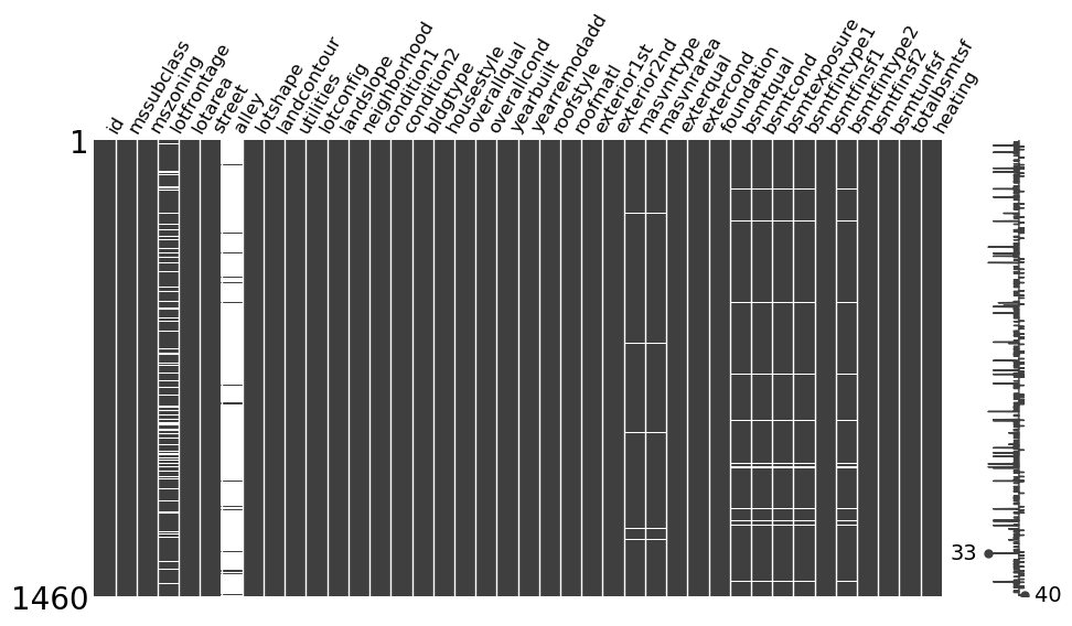
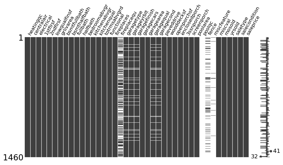
Overview

The output gives a visual overview of how many missing values each column has. It also shows in which rows the missing values occur and therefore lets one get an idea of which columns are correlated in terms of their rows with missing values.

Using the plot, we can investigate the following, in order to see if there is a pattern present for each column that has many missing values. While ‘many missing values’ is by no means a criterium to go by when filling missing values, there is no fits all type of solution when it comes to dealing with missing values.

Default Strategy

Let me explain why and how I determine which columns to manually fill, using custom fill values that are not the median of all non-missing values found in a column, if the column is of type numerical or the mode in case of a string column.

Early Benchmark

I like to use as little preprocessing as possible before training the first model, just enough that the data is ready for the model to be trained on. That way I get a first benchmark early. Most of the time I use a tree based model, that lets me evaluate the relative feature importances of the columns among other metrics that I look at. Only after this first iteration, will I think about if using custom fill values is likely to payoff in bettering the accuracy score, more than all the other preprocessing steps that could be added instead.

Examples Of Common Cases

For this article, in order to show how I would deal with the columns that have missing values, we look at the ones, where rows with missing values actually don’t mean that the value is missing - is unknown. This happens frequently, when the data is not properly collected for that feature with missing values. E.g., column poolqc, which stands for ‘pool quality’.

We create the function bivar that accepts two columns of a DataFrame, related_col and missing_col and returns the unique values for the pair of the two columns, only using the rows where missing_col has missing values.

def bivar(related_col, missing_col):
    missing_rows = train[[related_col, missing_col]][train[missing_col].isna() == True]
    uniques = {related_col: [], missing_col: []}
    for key in uniques.keys():
        uniques[key].append(missing_rows[key].unique())
    print(uniques)

Case: A Category Is Missing

The output for poolarea and poolqc shows that only rows with missing values in poolqc are found, if and only if column poolarea has value 0 in the same row. A value of 0 means that the listing has no pool and therefore no poolqc. The values are not missing in this case, instead a new class should be added to the ones present in the column. It could be something like ‘no_pool’.

bivar("poolarea", "poolqc")

{'poolarea': [array([0])], 'poolqc': [array([nan], dtype=object)]}

The same relationship is found for column fireplacequ, which categorizes the quality of a fireplace if the particular house has a fireplace.

bivar("fireplaces", "fireplacequ")

{'fireplaces': [array([0])], 'fireplacequ': [array([nan], dtype=object)]}

Case: Default Fill Values

Column alley uses nan values where neither a gravel nor a pave alley is found. A new category, like ‘no_alley’ could be used to fill the missing values here.

train.alley.unique()

array([nan, 'Grvl', 'Pave'], dtype=object)

Variable lotfrontage measures the Lot Frontage, which is a legal term. Without getting too specific, it measures the portion of a lot abutting a street. It is unclear, whether the nan values in this column are not just actual nan values. In this case I would prefer to use the median of all non-missing values in the column, to fill the missing values.

train.lotfrontage.unique()

array([ 65.,  80.,  68.,  60.,  84.,  85.,  75.,  nan,  51.,  50.,  70.,
        91.,  72.,  66., 101.,  57.,  44., 110.,  98.,  47., 108., 112.,
        74., 115.,  61.,  48.,  33.,  52., 100.,  24.,  89.,  63.,  76.,
        81.,  95.,  69.,  21.,  32.,  78., 121., 122.,  40., 105.,  73.,
        77.,  64.,  94.,  34.,  90.,  55.,  88.,  82.,  71., 120., 107.,
        92., 134.,  62.,  86., 141.,  97.,  54.,  41.,  79., 174.,  99.,
        67.,  83.,  43., 103.,  93.,  30., 129., 140.,  35.,  37., 118.,
        87., 116., 150., 111.,  49.,  96.,  59.,  36.,  56., 102.,  58.,
        38., 109., 130.,  53., 137.,  45., 106., 104.,  42.,  39., 144.,
       114., 128., 149., 313., 168., 182., 138., 160., 152., 124., 153.,
        46.])

For variable fence, I would use the mode, since there is no indication that the nan values are not just missing values.

train.fence.unique()

array([nan, 'MnPrv', 'GdWo', 'GdPrv', 'MnWw'], dtype=object)

The examples cover many of the cases that can happen and show for each of the most common types how I would fill the missing values. A more in-depth analysis and a custom fill strategy can be necessary, if the particular column is of high importance and therefore justifies a complex filling strategy.

Categorical Embeddings

The goal is to create categorical embeddings that will transform the categorical string variables into ordered categorical type columns. For this, we are looking for columns whose unique values have an inherent order that we can use to make the transformation using the pandas library. While categorical embeddings don’t make a difference for tree ensembles, they do for deep learning models that unlike tree based models can make use of the added information given by categorical embeddings for categorical variables.

Find Candidate Columns

The output below shows that there are three types of data types currently assigned to the columns of train. The ones with dtype object are the ones we focus on here in the following step.

def guc(train: pd.DataFrame, p=None):
    dts = [train[c].dtype for c in train.columns]
    ut, uc = np.unique(dts, return_counts=True)
    if p == True:
        for i in range(len(ut)):
            print(ut[i], uc[i])

    return ut, uc

_, _ = guc(train, p=True)

int64 34
float64 4
object 43

The function below returns a dictionary of column name and list of unique values for all columns that have less than ul unique values and that are of type ‘object’ by default. The input parameters can be altered to filter for columns with less or more number of unique values than the default value and one can look for other column data types as well.

def can(train=train, ul=13, tp="object"):
    dd = [
        (c, train[c].unique())
        for c in train.columns
        if train[c].nunique() < ul and train[c].dtype == tp
    ]
    ddc = dict(dd)
    return ddc

ddc = can()
ddc

{'mszoning': array(['RL', 'RM', 'C (all)', 'FV', 'RH'], dtype=object),
 'street': array(['Pave', 'Grvl'], dtype=object),
 'alley': array([nan, 'Grvl', 'Pave'], dtype=object),
 'lotshape': array(['Reg', 'IR1', 'IR2', 'IR3'], dtype=object),
 'landcontour': array(['Lvl', 'Bnk', 'Low', 'HLS'], dtype=object),
 'utilities': array(['AllPub', 'NoSeWa'], dtype=object),
 'lotconfig': array(['Inside', 'FR2', 'Corner', 'CulDSac', 'FR3'], dtype=object),
 'landslope': array(['Gtl', 'Mod', 'Sev'], dtype=object),
 'condition1': array(['Norm', 'Feedr', 'PosN', 'Artery', 'RRAe', 'RRNn', 'RRAn', 'PosA',
        'RRNe'], dtype=object),
 'condition2': array(['Norm', 'Artery', 'RRNn', 'Feedr', 'PosN', 'PosA', 'RRAn', 'RRAe'],
       dtype=object),
 'bldgtype': array(['1Fam', '2fmCon', 'Duplex', 'TwnhsE', 'Twnhs'], dtype=object),
 'housestyle': array(['2Story', '1Story', '1.5Fin', '1.5Unf', 'SFoyer', 'SLvl', '2.5Unf',
        '2.5Fin'], dtype=object),
 'roofstyle': array(['Gable', 'Hip', 'Gambrel', 'Mansard', 'Flat', 'Shed'], dtype=object),
 'roofmatl': array(['CompShg', 'WdShngl', 'Metal', 'WdShake', 'Membran', 'Tar&Grv',
        'Roll', 'ClyTile'], dtype=object),
 'masvnrtype': array(['BrkFace', 'None', 'Stone', 'BrkCmn', nan], dtype=object),
 'exterqual': array(['Gd', 'TA', 'Ex', 'Fa'], dtype=object),
 'extercond': array(['TA', 'Gd', 'Fa', 'Po', 'Ex'], dtype=object),
 'foundation': array(['PConc', 'CBlock', 'BrkTil', 'Wood', 'Slab', 'Stone'], dtype=object),
 'bsmtqual': array(['Gd', 'TA', 'Ex', nan, 'Fa'], dtype=object),
 'bsmtcond': array(['TA', 'Gd', nan, 'Fa', 'Po'], dtype=object),
 'bsmtexposure': array(['No', 'Gd', 'Mn', 'Av', nan], dtype=object),
 'bsmtfintype1': array(['GLQ', 'ALQ', 'Unf', 'Rec', 'BLQ', nan, 'LwQ'], dtype=object),
 'bsmtfintype2': array(['Unf', 'BLQ', nan, 'ALQ', 'Rec', 'LwQ', 'GLQ'], dtype=object),
 'heating': array(['GasA', 'GasW', 'Grav', 'Wall', 'OthW', 'Floor'], dtype=object),
 'heatingqc': array(['Ex', 'Gd', 'TA', 'Fa', 'Po'], dtype=object),
 'centralair': array(['Y', 'N'], dtype=object),
 'electrical': array(['SBrkr', 'FuseF', 'FuseA', 'FuseP', 'Mix', nan], dtype=object),
 'kitchenqual': array(['Gd', 'TA', 'Ex', 'Fa'], dtype=object),
 'functional': array(['Typ', 'Min1', 'Maj1', 'Min2', 'Mod', 'Maj2', 'Sev'], dtype=object),
 'fireplacequ': array([nan, 'TA', 'Gd', 'Fa', 'Ex', 'Po'], dtype=object),
 'garagetype': array(['Attchd', 'Detchd', 'BuiltIn', 'CarPort', nan, 'Basment', '2Types'],
       dtype=object),
 'garagefinish': array(['RFn', 'Unf', 'Fin', nan], dtype=object),
 'garagequal': array(['TA', 'Fa', 'Gd', nan, 'Ex', 'Po'], dtype=object),
 'garagecond': array(['TA', 'Fa', nan, 'Gd', 'Po', 'Ex'], dtype=object),
 'paveddrive': array(['Y', 'N', 'P'], dtype=object),
 'poolqc': array([nan, 'Ex', 'Fa', 'Gd'], dtype=object),
 'fence': array([nan, 'MnPrv', 'GdWo', 'GdPrv', 'MnWw'], dtype=object),
 'miscfeature': array([nan, 'Shed', 'Gar2', 'Othr', 'TenC'], dtype=object),
 'saletype': array(['WD', 'New', 'COD', 'ConLD', 'ConLI', 'CWD', 'ConLw', 'Con', 'Oth'],
       dtype=object),
 'salecondition': array(['Normal', 'Abnorml', 'Partial', 'AdjLand', 'Alloca', 'Family'],
       dtype=object)}

The output of the function shows that there are many columns that could be good candidates for categorical embeddings. We look for ones that have a clear inherent ordering and that can be batch processed.

Criteria

Using the output of the function above, the unique values of all columns of type object are screened for ones that have an intrinsic ordering. One could spend more time finding additional columns with ordered values of type object or also including columns with unique values of other types, e.g., see the output of the can function above. The goal here was to find several columns that meet this criterium that can be batch processed without the need to individually set the ordered categorical dtype for each column, since the unique values of the columns don’t share close to the same set of unique values that all follow the same order.

Unique Values

The unique values below are found in several string columns, follow the same ordering and are almost identical. The abbreviations are listed in the table below. The placement within the order of each set of unique values for each column depends on whether there are missing values present in the value range of the particular column. This is indicated by the values of column Condition For Rank in the table below. Only the relative rank of each class within the values found in a specific column is relevant, e.g., whether the order of “Po” is the lowest (0) or (1), second lowest, does not matter for the actual transformation.

Order	Abbreviation	Category	Condition For Rank
0	“FM”	false or missing (`nan`)	-
0	None	missing value (`nan`)	-
0/1	“Po”	poor	-+ `nan`
1/2	“Fa”	fair	-+ `nan`
2/3	“TA”	typical/average	-+ `nan`
3/4	“Gd”	good	-+ `nan`
4/5	“Ex”	excellent	-+ `nan`

The Transformation

Three different variations of the value range are found and specified below in ascending order from left to right.

uset = ["Po", "Fa", "TA", "Gd", "Ex"]
usetNA = [None, "Po", "Fa", "TA", "Gd", "Ex"]
usetna = ["FM", "Po", "Fa", "TA", "Gd", "Ex"]

The function cu does the transformation for all three cases.

def cu(df: pd.DataFrame, uset: list, usetna: list):
    cols = [
        (c, df[c].unique().tolist())
        for c in df.columns.tolist()
        if df[c].dtype == "object" and set(df[c].unique()).issuperset(uset)
    ]
    for cc in cols:
        # name of the column, as filtered by list comprehension cols
        name = cc[0]
        vals = uset
        valsna = usetna
        # fill missing values with string "FM" - false or missing
        df[name].fillna(value="FM", inplace=True)
        # change column to dtype category
        df[name] = df[name].astype("category")
        # no missing values and no FM category indicating missing values.
        if set(df[name].unique()) == set(uset):
            # unique values are not changed in this case.
            vals = vals
            # dtype changed to ordered categorical.
            df[name].cat.set_categories(vals, ordered=True, inplace=True)
            # print name of column, followed by its ordered categories.
            print(name, df[name].cat.categories)
        # missing values present, as indicated by category "FM"
        elif set(df[name].unique()) == set(usetna):
            valsna = valsna
            df[name].cat.set_categories(valsna, ordered=True, inplace=True)
            # print name of column, followed by its ordered categories.
            print(name, df[name].cat.categories)
    return df

We pass the function the training dataset and the three value ranges to filter on and update the train DataFrame with the output of function cu.

train = cu(train, uset, usetna)

extercond Index(['Po', 'Fa', 'TA', 'Gd', 'Ex'], dtype='object')
heatingqc Index(['Po', 'Fa', 'TA', 'Gd', 'Ex'], dtype='object')
fireplacequ Index(['FM', 'Po', 'Fa', 'TA', 'Gd', 'Ex'], dtype='object')
garagequal Index(['FM', 'Po', 'Fa', 'TA', 'Gd', 'Ex'], dtype='object')
garagecond Index(['FM', 'Po', 'Fa', 'TA', 'Gd', 'Ex'], dtype='object')

Final Preprocessing: TabularPandas

Often times I tend to use function train_test_split from sklearn, after manually doing all the preprocessing. In this case, we use function TabularPandas (TabularPandas Documentation) from library fastai, which is a convenient wrapper around several preprocessing functions that transform a DataFrame.

procs = [Categorify, FillMissing]
dep_var = "saleprice"
cont, cat = cont_cat_split(df=train, max_card=1, dep_var=dep_var)
train_s, valid_s = RandomSplitter(seed=42)(train)
to = TabularPandas(
    train,
    procs,
    cat,
    cont,
    y_names=dep_var,
    splits=(train_s, valid_s),
    reduce_memory=False,
)

Explanation Of Parameter Choices

For the train DataFrame we specify the following parameters and add a description of what each one does.

procs

We specify [Categorify, FillMissing] for this parameter. What that does is apply two transformations to the entire input DataFrame. Categorify will transform categorical variables to numerical values and will respect ones that are already of type ordered categorical. The documentation can be found here: Categorify Documentation. FillMissing will only target numerical columns and use the median as fill value by default. One can find its documentation following this link: FillMissing Documentation. Another transformation it does is add a new column for every column with missing values that indicates for each row in the dataset whether the value in that column was filled or not. It does so by adding a boolean type column for every column with missing values. E.g., see the output of the command below.

xs, y = to.train.xs, to.train.y  # defined here to show output of next line.
xs.filter(like="_na", axis=1).sample(n=5, random_state=seed)

	lotfrontage_na	masvnrarea_na	garageyrblt_na
465	2	1	1
77	1	1	1
1429	2	1	1
574	1	1	1
73	1	1	1

Parameter dep_var tells TabularPandas, which column(s) to use as the dependent variable(s).

cont, cat are the outputs of function cont_cat_split (cont_cat_split Documentation), which will assign each column to either type continuous or type categorical based on the threshold (max_card) passed for the maximum number of unique values that a column may have to still be classified as being categorical. In this case, since the preprocessing is only used to train tree ensemble models, there is no added information for the model, if we tell it that there are continuous, as well as categorical variables. This will change later, when we train a neural network, there the distinction is relevant.

train_s, valid_s are assigned the output of function RandomSplitter which splits the dataset along the row index into training and test data (valid_s). The default is 80 percent of rows are used for the training set, with the remaining 20 percent used for the test set. One can specify the argument seed in order to get the same split across several executions of the code.

In order to see the transformations done by calling TabularPandas, one has to use the variable assigned to the output of TabularPandas, to in this case. Like that, one can access several attributes of the created object, such as the following.

Get the length of the training and test set.

len(to.train), len(to.valid)

(1168, 292)

Print the classes behind the now numerical unique values of categorical type columns.

to.classes["heatingqc"]

['#na#', 'Po', 'Fa', 'TA', 'Gd', 'Ex']

to.classes["saletype"]

['#na#', 'COD', 'CWD', 'Con', 'ConLD', 'ConLI', 'ConLw', 'New', 'Oth', 'WD']

to["saletype"].unique()

array([9, 7, 1, 2, 8, 4, 6, 5, 3], dtype=int8)

to.items.head()

	id	mssubclass	mszoning	lotfrontage	lotarea	...	salecondition	saleprice	lotfrontage_na	masvnrarea_na	garageyrblt_na
1172	1173	160	2	35.0	4017	...	5	12.054668	1	1	1
1313	1314	60	4	108.0	14774	...	5	12.716402	1	1	1
1327	1328	20	4	60.0	6600	...	5	11.779129	1	1	1
29	30	30	5	60.0	6324	...	5	11.134589	1	1	1
397	398	60	4	69.0	7590	...	5	12.040608	1	1	1

5 rows × 84 columns

Once the preprocessing is done, one can save the resulting object to a pickle file like shown below.

save_pickle("top.pkl", to)

Entire Series: