Decision Tree Feature Selection Methodology, Part 2

Detailed exploration of feature selection using sklearn's DecisionTreeRegressor. It includes testing the reliability of the feature_importances_ method.

Tags: decision-tree-analysis feature-selection-techniques sklearn model-evaluation tabular-data

Category: Tabular Data

Series: Kaggle Competition - Deep Dive Tabular Data

Advanced Missing Value Analysis in Tabular Data, Part 1
Decision Tree Feature Selection Methodology, Part 2
RandomForestRegressor Performance Analysis, Part 3
Statistical Interpretation of Tabular Data, Part 4
Addressing the Out-of-Domain Problem in Feature Selection, Part 5
Kaggle Challenge Strategy: RandomForestRegressor and Deep Learning, Part 6
Hyperparameter Optimization in Deep Learning for Kaggle, Part 7

Decision Tree Feature Selection Methodology, Part 2

With the preprocessing done, we can start with the machine learning. However, this is not the type of machine learning where we look for the highest accuracy we can get, given a model architecture and hyperparameters. In this case we are looking to get a better understanding of which of the 80 independent variables contribute most to the final predictions that the fitted model makes and how.

Train & Validation Splits

We will always use to.train.xs and to.train.y to assign the training pair of independent variables and dependent variable. In the same way, we will always assign the test pair.

xs, y = to.train.xs, to.train.y
valid_xs, valid_y = to.valid.xs, to.valid.y

Sklearn DecisionTreeRegressor

The first model used is a simple decision tree model that we will use to see what columns and values the model uses to create the splits. Plus, we like to see the order of the splits that the model chooses. From library scikit-learn we use the DecisionTreeRegressor model (DecisionTreeRegressor Documentation).

Feature Selection

Since we are looking for eliminate irrelevant variables (features), we tell it to only consider at maximum 40 of the 80 columns when deciding which feature is the best one to use for the next split. The model must not create leaves that have less than 50 samples for the final split. The model is fit using the train split we created earlier.

m = DecisionTreeRegressor(max_features=40, min_samples_leaf=50, random_state=seed)
m.fit(xs, y)

DecisionTreeRegressor(max_features=40, min_samples_leaf=50, random_state=42)

In a Jupyter environment, please rerun this cell to show the HTML representation or trust the notebook.
On GitHub, the HTML representation is unable to render, please try loading this page with nbviewer.org.

DecisionTreeRegressor Visualization Examples

Two visualization tools are used to visualize the splits of the fitted model. The first one is a rather basic one, while dtreeviz is a more detailed visualization.

ax, fig = plt.subplots(1, 1, figsize=(18, 12))
ax = plt.subplot(111)
plot_tree(m, feature_names=[c for c in xs.columns if c != "saleprice"],
          ax=ax,fontsize=6)
plt.savefig(f"plot_tree-1", dpi=300,bbox_inches='tight')

sklearn plot_tree

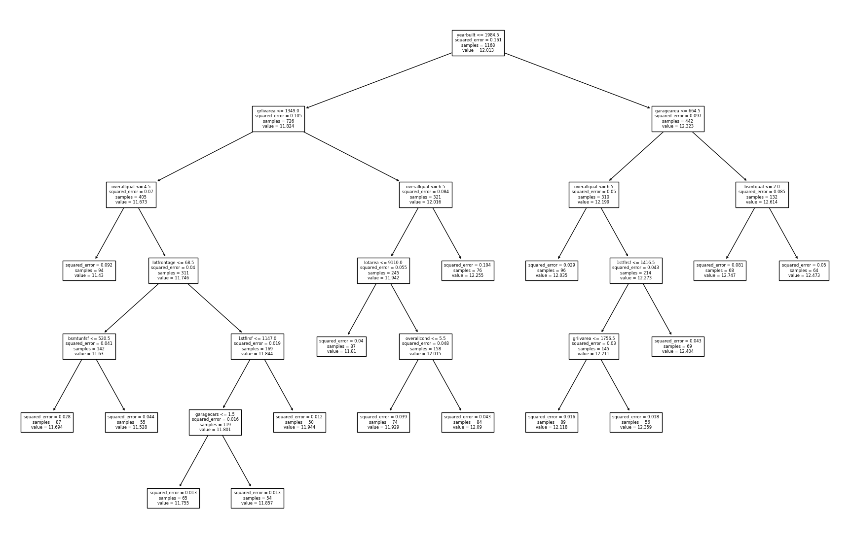
fig = plt.figure(figsize=(22, 14))

dtreeviz(
    m,
    xs,
    y,
    xs.columns,
    dep_var,
    fontname="DejaVu Sans",
    scale=1.1,
    label_fontsize=11,
    orientation="LR",
)

dtreeviz visualization

Theory

A reason why tree based models are one of the best model types when it comes to understanding the model and the splits a fitted model created lies in the fact, that there is a good infrastructure for this type of model when it comes to libraries and functions created for that purpose. That and the fact that this type of model has a transparent and fairly easy to understand structure. The tree based models we use for understanding are ones, where the tree or the trees in the case of the RandomForestRegressor are intentionally kept weak. This is not necessarily the case for the DecisionTreeRegressor model, since without limiting the number of splits, there is no mechanism to limit the size of the final tree. While the size of the DecisionTreeRegressor can be limited by use of its parameters to combat overfitting, it is the RandomForestRegressor model that is the preferred model from the two when it comes to the feature_importances_ metric. A metric used for feature selection and for understanding the relative importance that each feature has. Both models feature this method.

Feature Importance Relative Metric

From the scikit-learn website, one gets the following definition for the feature_importances_ attribute:

property feature_importances_
Return the feature importances. The importance of a feature is computed as the (normalized) total reduction of the criterion brought by that feature. It is also known as the Gini importance.

Definition of feature_importances_ attribute on scikit-learn

fi = dict(zip(train.columns.tolist(), m.feature_importances_))

Feature Selection Using Features Importance Scores

Using the feature importances values, we can set a lower limit for the feature importance score. All features with a feature importance lower than the threshold are dropped from the train dataset and saved as a new DataFrame for illustration purposes. Only the ones are kept that a features importance score larger zero. The result is a subset of 11 columns of the original 80 columns.

fip = pd.DataFrame(fi, index=range(0, 1))
fipl = fip[fip > 0].dropna(axis=1).T.sort_values(by=0, ascending=False)
fipl.rename(columns={0: "feature_importance"}, inplace=True)
fipl

	feature_importance
kitchenabvgr	0.498481
garagearea	0.168625
halfbath	0.121552
...	...
bedroomabvgr	0.007406
fireplacequ	0.006791
poolqc	0.002268

11 rows × 1 columns

Feature Importance Metric Deep Dive Experiment

It was unclear, whether the order from most important feature to the ones with a feature importance score of zero according to the feature_importances_ method changes between executions, using the same parameters and data to train the DecisionTreeRegressor estimator. Changes in the subset of columns that have a feature importance score larger zero led to inconsistencies and ultimately errors when the same code was executed repeatedly. This was observed while using the same random_state seed to ensure that the output of functions generating and using pseudo random numbers stayed the same across different executions.

Another possibility is that the feature importance scores change and ultimately reorder the ranking of the columns based on these scores in some cases. These deviations might however be the result of changes in the model parameters by the user between executions, rather than returning differing values across multiple executions without any interactions by the user.

To answer this question, an experiment is conducted where 1000 DecisionTreeRegressor estimators are trained and the feature_importances_ method is used to get and log the feature importance score for each feature during each of the 1000 samples. The results are then averaged, and the standard deviation calculated for each feature over the 2000 samples.

With the results, one can answer the research question of whether the feature_importances_ method itself is prone to generating inconsistent feature importance scores for the features used as independent variables during fitting of the DecisionTreeRegressor in this case. Using 1000 iterations will not only give a mean feature importance score $\hat{\mu}$ for each feature that is much closer to the true mean $\mu$, but also a value for the standard deviation $\hat{\sigma}$ for the sample. The following function does just that and creates two summary plots that visualize the final results and answers the research question.

In summary, the output shows that in this instance, there is no change in the order of the features as given by the feature_importances_ method. Further, there is no relevant deviation of the values assigned to each feature by the method, over the 1000 samples. The changes in the ordering, at least in this case must have come from the user changing parameter values in the creation of the RandomForestRegressor estimator.

m.feature_importances_

array([0.        , 0.        , 0.        , 0.        , 0.        ,
       0.        , 0.        , 0.        , 0.        , 0.        ,
       0.        , 0.        , 0.        , 0.        , 0.        ,
       0.        , 0.        , 0.        , 0.        , 0.        ,
       0.        , 0.018051  , 0.        , 0.        , 0.        ,
       0.        , 0.        , 0.        , 0.        , 0.        ,
       0.        , 0.        , 0.        , 0.        , 0.        ,
       0.        , 0.        , 0.        , 0.        , 0.        ,
       0.        , 0.        , 0.        , 0.        , 0.        ,
       0.        , 0.        , 0.        , 0.02573276, 0.01708777,
       0.12155166, 0.00740567, 0.49848064, 0.        , 0.        ,
       0.        , 0.        , 0.00679074, 0.        , 0.01795456,
       0.        , 0.        , 0.16862501, 0.        , 0.        ,
       0.        , 0.        , 0.        , 0.        , 0.        ,
       0.        , 0.        , 0.00226778, 0.11605241, 0.        ,
       0.        , 0.        , 0.        , 0.        , 0.        ,
       0.        , 0.        , 0.        ])

Test Setup - Create 1000 Samples

def fp(train=train, xs=xs, y=y, i=1):
    cc = train.columns.tolist()
    tup = [(c, []) for c in cc]
    msd = dict(tup)
    fpd = dict(tup)
    for t in range(i):
        mi = DecisionTreeRegressor(
            max_features=40, min_samples_leaf=50, random_state=seed
        )
        mi.fit(xs, y)
        fii = mi.feature_importances_
        for c, s in zip(cc, fii):
            fpd[f"{c}"].append(s)
    cc = train.columns.tolist()
    tup = [(c, []) for c in cc]
    msd = dict(tup)
    for i in fpd.keys():
        num = 0
        mean, std = np.mean(fpd[i]), np.std(fpd[i])
        msd[i].append(mean)
        msd[i].append(std)
        if num == 0:
            num = len(fpd[i])

    dffp = pd.DataFrame(msd).T.sort_values(by=0, ascending=False)
    dffpg0 = dffp[dffp.iloc[:, 0] > 0]
    cols_filter = dffpg0.reset_index()
    dffpdo =pd.DataFrame(fpd,columns=cols_filter['index'].tolist())
    fig, ax = plt.subplots(1,2,figsize=(22,10))
    ax=plt.subplot(121)
    dffpg0[0].plot(kind="barh", figsize=(12, 7), legend=False)
    plt.title(f"mean of {num} samples")
    plt.subplots_adjust(left=.14)
    plt.subplots_adjust(bottom=.2)
    plt.ylabel('features')
    plt.xlabel('relative feature importance, if greater 0')
    ax=plt.subplot(122)
    sns.boxplot(data=dffpdo,ax=ax)
    ax.set_title(f'Boxplot Of Feature Importances')
    plt.xticks(rotation=90)
    plt.show()

fpdo = fp(i=1000)

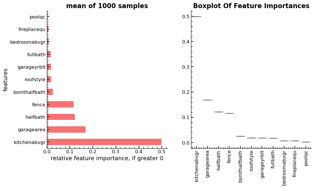
Left: Feature importance plot for features with feature importance score greater 0 over 1000 samples.
Right: Boxplot of 1000 samples, showing no change in rank and almost no deviations in scores across samples.

Entire Series: