RandomForestRegressor Performance Analysis, Part 3

In-depth analysis of RandomForestRegressor, focusing on feature importance and out-of-bag error as key performance indicators.

Tags: performance-analysis random-forest-optimization model-evaluation feature-importance tabular-data

Category: Tabular Data

Series: Kaggle Competition - Deep Dive Tabular Data

Advanced Missing Value Analysis in Tabular Data, Part 1
Decision Tree Feature Selection Methodology, Part 2
RandomForestRegressor Performance Analysis, Part 3
Statistical Interpretation of Tabular Data, Part 4
Addressing the Out-of-Domain Problem in Feature Selection, Part 5
Kaggle Challenge Strategy: RandomForestRegressor and Deep Learning, Part 6
Hyperparameter Optimization in Deep Learning for Kaggle, Part 7

RandomForestRegressor Performance Analysis, Part 3

Create Root Mean Squared Error Metric For Scoring Models

Given that the kaggle competition we want to submit our final predictions uses a root mean squared error as scoring metric, we create this metric for all future scoring of predictions.

def r_mse(pred, y):
    return round(math.sqrt(((pred - y) ** 2).mean()), 6)

def m_rmse(m, xs, y):
    return r_mse(m.predict(xs), y)

We score the fitted model on the training set, in order to be able to compare it to the predictions on the validation set. Only the predictions and the score on the validation dataset matter in the end.

m_rmse(m, xs, y)

0.207714

The model is scored on the validation set.

m_rmse(m, valid_xs, valid_y)

0.198003

Custom Function To Create And Fit A RFR Estimator

A function that creates a RandomForestRegressor estimator and fits it using the training data. Its output is the fitted estimator.

def rf(
    xs,
    y,
    n_estimators=30,
    max_samples=500,
    max_features=0.5,
    min_samples_leaf=5,
    **kwargs,
):
    return RandomForestRegressor(
        n_jobs=-1,
        n_estimators=n_estimators,
        max_samples=max_samples,
        max_features=max_features,
        min_samples_leaf=min_samples_leaf,
        oob_score=True,
        random_state=seed,
    ).fit(xs, y)

m = rf(xs, y)

m_rmse is used to calculate the mean squared error for the estimator on the training and validation set.

m_rmse(m, xs, y), m_rmse(m, valid_xs, valid_y)

(0.124994, 0.13605)

RFR - Theory

The RandomForestRegressor model uses a subset of the training set to train each decision tree in the ensemble on. The following parameter names are specific to the implementation in the sklearn library. The number of decision trees in the ensemble depends on the value of parameter n_estimators and the size of the subset is controlled by max_samples, given the default value of bootstrap=True. If bootstrap=False or max_samples=None, then each base estimator is trained using the entire training set. See RandomForestRegressor Documentation

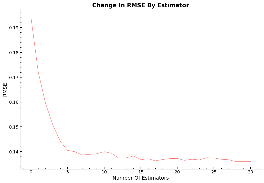
Given that each base base estimator was trained with a maximum of 500 samples or ~43% of all training samples, it is likely that the average of the RMSE over the predictions for the samples in the validation dataset is more volatile for a low number of estimators, and is less volatile as additional base estimators are added one by one, until all 30 are used and their predictions are averaged. We expect the value for the average RMSE over all 30 base estimators to be equal to the RMSE value we got when executing m_rmse(m, valid_xs, valid_y).

x=len(xs)
pct = np.ceil((500/x)*100)
print(f'Percentage of samples each base estimator uses of the training data: {pct}\n')
preds = np.stack([t.predict(valid_xs) for t in m.estimators_])
print(f'The mean RMSE over all trees on the validation dataset is: {r_mse(preds.mean(0), valid_y)}')

Percentage of samples each base estimator uses of the training data: 43.0

The mean RMSE over all trees on the validation dataset is: 0.13605

RFR - Average RMSE By Number Of Estimators

Visualization of the average RMSE value, by number of estimators added.

fig, ax = plt.subplots(1, 1, figsize=(8, 4))
ax = plt.subplot(111)
ax.plot([r_mse(preds[: i + 1].mean(0), valid_y) for i in range(31)])
ax.set_title("Change In RMSE By Estimator")
ax.set_xlabel("Number Of Estimators")
ax.set_ylabel("RMSE")
plt.show()

RMSE value on the training set, as base estimators are added one by one. Value is volatile for low number of estimators, less so as more estimators are added.

Out-Of-Bag Error Explained

In the case, where the size of the subset used to train each base estimator was smaller than the set of the training data, one can look at the out-of-bag error, as seen below. It is a metric one can use in addition to cross-validation to estimate the models performance on unseen data.

Out-of-bag error
The out-of-bag error is the mean error on each training sample, using only the trees whose training subset did not include that particular sample.

The value for the RMSE, only using out-of-bag samples is higher than the RMSE on the training and validation set, which was expected.

r_mse(m.oob_prediction_, y)

0.154057

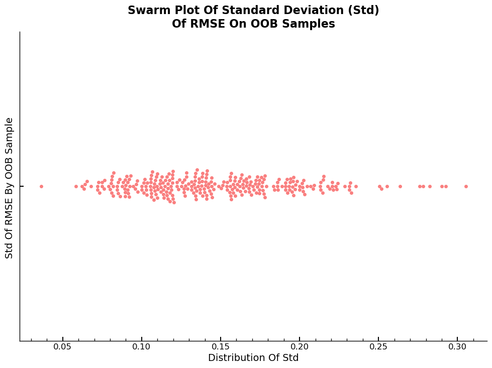
RFR: Standard Deviation Of RMSE By Number Of Estimators

We want to answer the following question:

How confident are we in our predictions using a particular row of data?

One can visualize the distribution of the standard deviation of the predictions over all estimators for each sample in the validation dataset. Given that estimator was trained on a subset of maximum 500 samples, the standard deviation can be relatively large for certain estimator sample combinations in the validation set. The average over all 30 base estimators however generalizes the final value for each sample in the validation set again and can be interpreted as the confidence in the predictions of the model for each sample. E.g., a low/high standard deviation for a particular sample means that the spread in the predicted sale price across all estimators is low/high and thus, the confidence of the model in the prediction is high/low.

Visualization Using Swarmplot

The values on the x-axis of the plot are \(\hat{\sigma}_{ln\,Y}\), with \(Y\) the random variable, the distribution of the standard deviation over all estimators for each sample in the validation dataset.

preds_std = np.sort(
    preds.std(0),
    axis=0,
)
fig, ax = plt.subplots(1,1,figsize=(6,5))
ax = plt.subplot(111)
sns.swarmplot(preds_std,orient='h',alpha=0.9,ax=ax)
ax.set_ylabel("Std Of RMSE By OOB Sample ")
ax.set_xlabel("Distribution Of Std")
ax.set_title(f'Swarm Plot Of Standard Deviation (Std)\nOf RMSE On OOB Samples')
plt.show()

Feature Importances And Selection Using RFR

The dataset used here has 80 independent variables, of which most are assigned 0, which means that their respective contribution, relative to the other features in terms of lowering the overall RMSE value is non-existent, judging by the feature_importances_ method. The underlying metric is the Gini importance metric, as mentioned earlier.

Compute Feature Importance Scores

A function is created that calculates the feature importances and returns a sorted DataFrame.

def rf_feat_importance(m, df):
    return pd.DataFrame(
        {"cols": df.columns, "imp": m.feature_importances_}).sort_values("imp", ascending=False)

Display The Top 10

We call the function and display the 10 features with the highest feature importance scores.

fi = rf_feat_importance(m, xs)
fi[:10]

	cols	imp
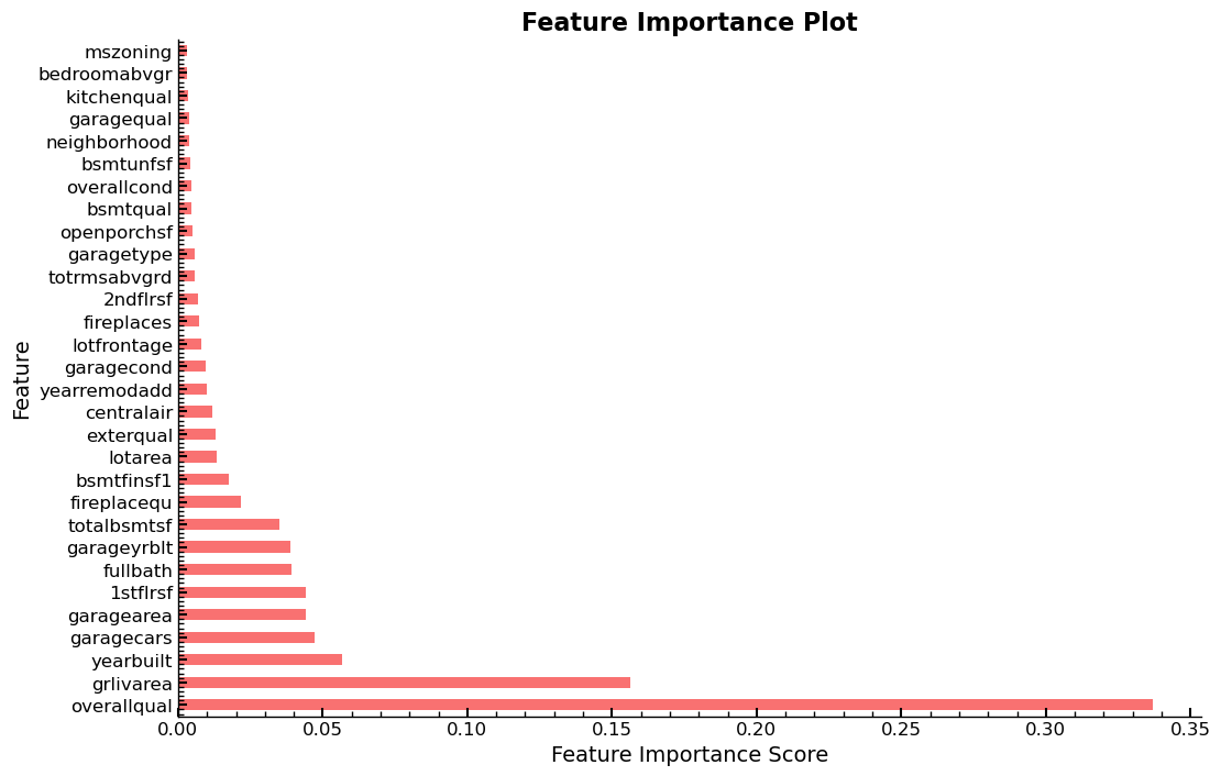
50	overallqual	0.336823
62	grlivarea	0.156380
52	yearbuilt	0.056838
...	...	...
71	garageyrblt	0.038850
58	totalbsmtsf	0.035039
32	fireplacequ	0.021616

10 rows × 2 columns

Bar Plot: Feature Importances

Function for the visualization of feature importance scores.

def plot_fi(fi):
    return fi.plot("cols", "imp", "barh", figsize=(12, 7), legend=False,title='Feature Importance Plot',ylabel='Feature',xlabel='Feature Importance Score')

Display The Top 30

Visualization of the 30 features, with the highest feature importance scores in ascending order.

plot_fi(fi[:30])

<AxesSubplot: title={'center': 'Feature Importance Plot'}, xlabel='Feature Importance Score', ylabel='Feature'>

Create Subset Of Features To Keep

We try to answer the following question:

Which columns are effectively redundant with each other, for purposes of prediction?

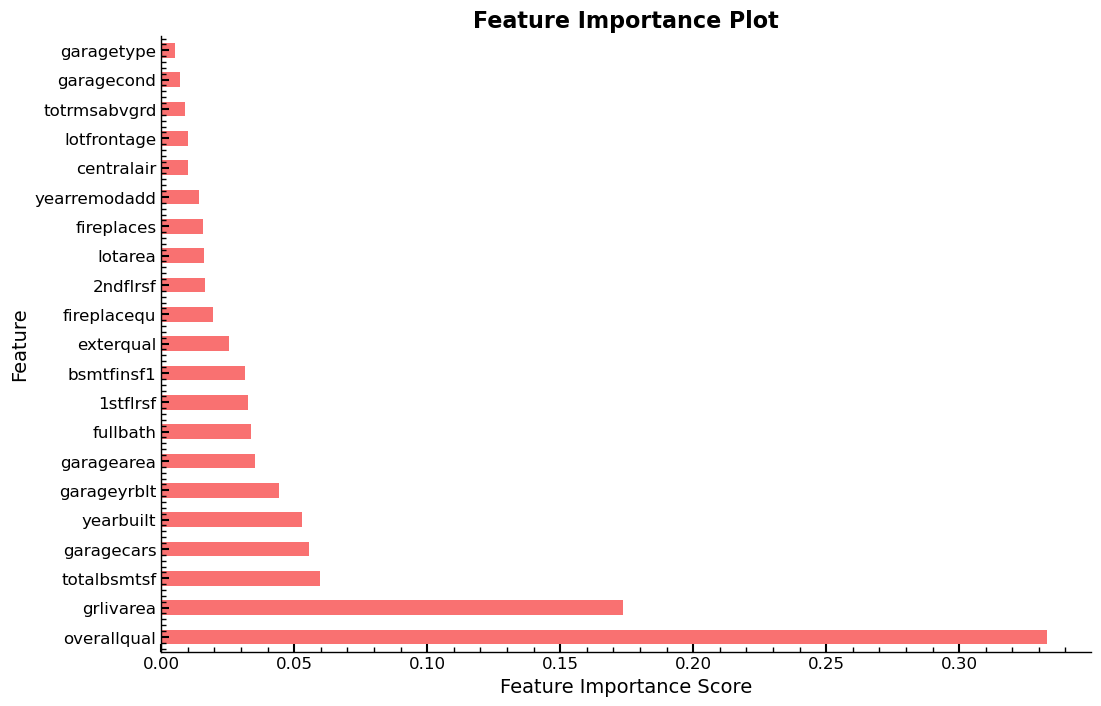
An arbitrary cutoff value of 0.005 is used, and only column names of features with a feature importance score larger 0.005 are kept. The number of columns that remain in the subset is printed.

to_keep = fi[fi.imp > 0.005].cols
len(to_keep)

New Training Set xs_imp After Feature Elimination

xs_imp/valid_xs_imp is the subset of xs/valid_xs with the columns that are in to_keep.

xs_imp = xs[to_keep]
valid_xs_imp = valid_xs[to_keep]

A RandomForestRegressor is fitted using xs_imp.

m = rf(xs_imp, y)

RMSE Values Using xs_imp

We want to answer this question:

How do predictions change, as we drop subsets of the features?

The RMSE values for the predictions on the training and validation dataset.

m_rmse(m, xs_imp, y), m_rmse(m, valid_xs_imp, valid_y)

(0.13191, 0.139431)

Interpretation Of RMSE Values

The RMSE values for the smaller feature set are worse compared to the ones using all features. In this case, this is a problem, given that kaggle scores our submission only on the RMSE value of the test set. In reality, this might be different. A model has to predict the sale price for houses it has never seen and not only on the kaggle test set. The predictions might be more robust and easier to interpret, given a smaller set of features.

len(xs.columns), len(xs_imp.columns)

(83, 21)

As a result of using xs_imp instead of xs and thus a smaller set of features, the feature importances can

plot_fi(rf_feat_importance(m, xs_imp))

<AxesSubplot: title={'center': 'Feature Importance Plot'}, xlabel='Feature Importance Score', ylabel='Feature'>

Entire Series: