Addressing the Out-of-Domain Problem in Feature Selection, Part 5

Comprehensive exploration of feature importance in tackling the out-of-domain problem, including identification, significance, and mitigation strategies.

Series: Kaggle Competition - Deep Dive Tabular Data

Advanced Missing Value Analysis in Tabular Data, Part 1
Decision Tree Feature Selection Methodology, Part 2
RandomForestRegressor Performance Analysis, Part 3
Statistical Interpretation of Tabular Data, Part 4
Addressing the Out-of-Domain Problem in Feature Selection, Part 5
Kaggle Challenge Strategy: RandomForestRegressor and Deep Learning, Part 6
Hyperparameter Optimization in Deep Learning for Kaggle, Part 7

Addressing the Out-of-Domain Problem in Feature Selection, Part 5

Introduction

The “out of domain” problem refers to the challenge of deploying machine learning models in real-world scenarios where the data distribution differs significantly from the data on which the model was trained. When a machine learning model is trained on a specific dataset, it learns to identify patterns and make predictions based on that dataset. However, when the model is deployed on a new dataset that is outside its training distribution, its performance can be severely impacted, resulting in lower accuracy and reliability.

The out of domain problem is especially relevant in industry projects where machine learning models are used to make critical business decisions. For example, in the finance industry, machine learning models are often used to identify fraud or predict credit risk. In these scenarios, the models must be highly accurate and reliable, and any errors can have serious consequences. If the model is trained on a dataset that is not representative of the real-world data, it can lead to false positives or false negatives, which can result in significant financial losses or damage to the reputation of the company.

Addressing the out of domain problem is therefore crucial for the success of machine learning projects in industry. One approach is to use transfer learning, where a pre-trained model is fine-tuned on the new dataset to adapt to the new distribution. Another approach is to use domain adaptation techniques, where the model is adapted to the new domain by modifying the feature space or the decision boundaries.

There has been significant research in recent years on addressing the out of domain problem in machine learning, with various techniques proposed to improve the generalization and robustness of machine learning models. Some notable research papers in this area include the following"Unsupervised Domain Adaptation by Backpropagation" by Ganin and Lempitsky"Domain-Adversarial Training of Neural Networks" by Tzeng et al."Deep Domain Confusion: Maximizing for Domain Invariance" by Ghifary et al..

Understanding and Addressing the Out-of-Domain Problem in Machine Learning

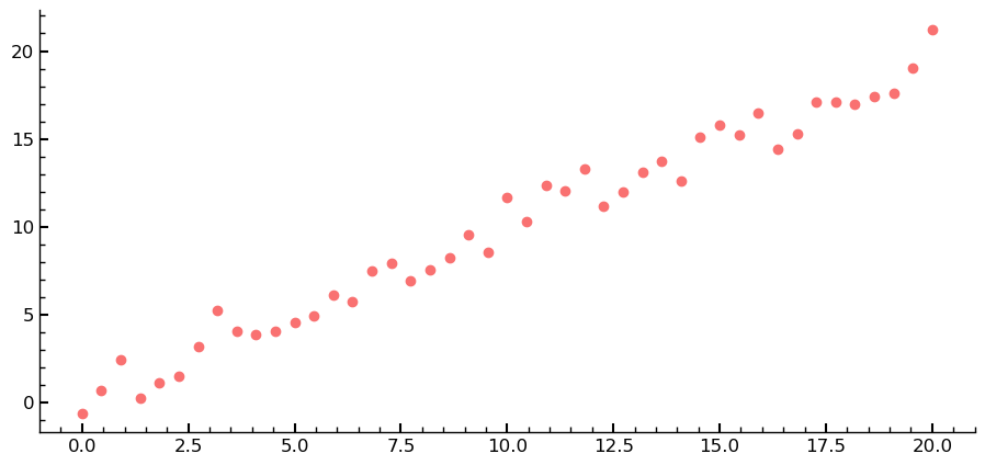
The provided code creates a series of 45 linear values for the x-axis and generates corresponding y-values by adding noise sampled from a normal distribution. The resulting data points are then plotted using a scatter plot.

xlins = torch.linspace(0, 20, steps=45)
ylins = xlins + torch.randn_like(xlins)
plt.scatter(xlins, ylins)

However, in order to train an estimator on this data, a second axis is needed. This can be achieved by using the .unsqueeze method or slicing the xslins variable using None.

xslins = xlins.unsqueeze(1)
xlins.shape, xslins.shape

(torch.Size([45]), torch.Size([45, 1]))

xlins[:, None].shape

torch.Size([45, 1])

Two different regression models, the RandomForestRegressor and XGBRegressor, are then trained on the first 35 rows of xslins and ylins.

m_linrfr = RandomForestRegressor().fit(xslins[:35], ylins[:35])
# Do the same and train a `XGBRegressor` using the same data.
m_lin = XGBRegressor().fit(xslins[:35], ylins[:35])

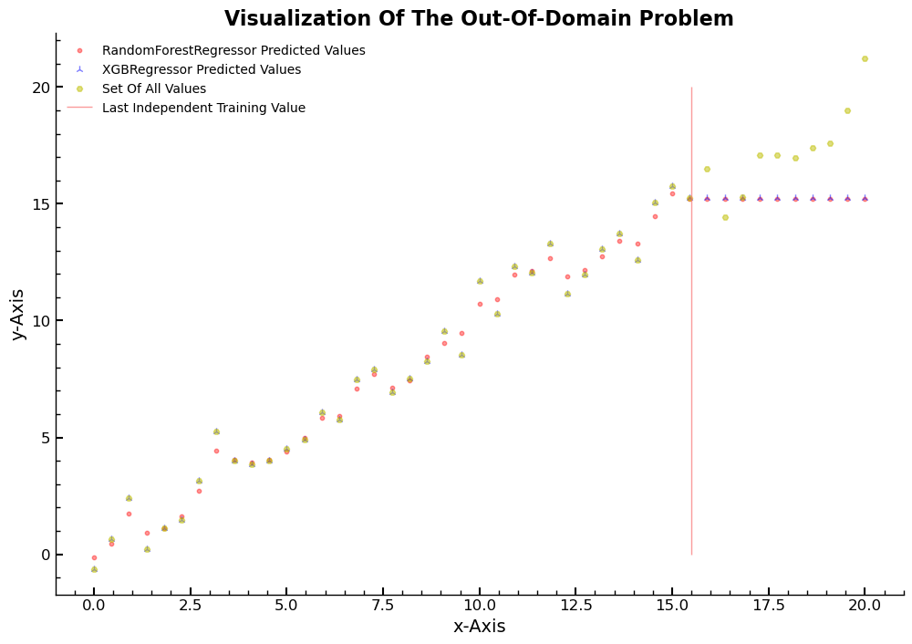
The scatter plot shows the predicted values for all points in xslins, as well as the final five values that were not used in the training data. The predicted values for the omitted values are all too low, highlighting the problem of the out-of-domain problem. This is an example of an extrapolation problem, where the model can only make predictions within the range of what it has seen for the dependent variable during training.

plt.scatter(xlins, m_linrfr.predict(xslins), c="r", alpha=0.4,s=10,label='RandomForestRegressor Predicted Values')
plt.scatter(xlins, m_lin.predict(xslins), c="b",marker="2", alpha=0.5,label='XGBRegressor Predicted Values')
plt.scatter(xslins, ylins, 20,marker="H",alpha=0.5, c="y",label='Set Of All Values')
plt.vlines(x=15.5,ymin=0,ymax=20,alpha=0.7,label='Last Independent Training Value')
plt.title('Visualization Of The Out-Of-Domain Problem')
plt.legend(loc='best')
plt.xlabel('x-Axis')
plt.ylabel('y-Axis')

Text(0, 0.5, 'y-Axis')

The reason behind this problem lies in the structure of the RandomForestRegressor and XGBRegressor models. These models average the predictions of several trees for each sample in the training data, and each tree averages the values of the dependent variable for all samples in a leaf. This approach can lead to predictions on out-of-domain data that are systematically too low. To avoid this issue, it is important to ensure that the validation set does not contain such data.

This out-of-domain problem is a critical issue in machine learning and has important implications for industry projects where machine learning models are used to make critical business decisions. Researchers have proposed various techniques, such as domain adaptation and transfer learning, to address this problem and improve the generalization and robustness of machine learning models, as discussed in the literatureGanin, Y., & Lempitsky, V. (2015). Unsupervised domain adaptation by backpropagation. In International Conference on Machine Learning (pp. 1180-1189).Tzeng, E., Hoffman, J., Saenko, K., & Darrell, T. (2017). Adversarial discriminative domain adaptation. In Proceedings of the IEEE Conference on Computer Vision and Pattern Recognition (pp. 7167-7176).Ghifary, M., Kleijn, W. B., Zhang, M., Balduzzi, D., & Li, W. (2016). Deep domain confusion: Maximizing for domain invariance. arXiv preprint arXiv:1412.3474.

Identifying Out-of-Domain Data with RandomForestRegressor

This section describes how to use the RandomForestRegressor tool to identify out-of-domain data. First, the train and validation data are merged, and a new dependent variable column is added to indicate whether the value of the dependent variable is part of the train or validation set. Then, the RandomForestRegressor is used to predict whether a row is part of the train or validation set.

Using the RandomForestRegressor, the feature importance of the dataset is computed, and the top eight most important features are identified. To determine which features can be dropped without losing accuracy, the RMSE value is calculated after dropping each of the top eight most important features. It is observed that dropping the garagearea feature does not decrease accuracy, but dropping garageyrblt does. Therefore, only garagearea is dropped.

The final RMSE value is then printed, which indicates the accuracy of the model on the validation set.

This process is important for ensuring the accuracy and reliability of machine learning models in identifying out-of-domain data, which can lead to incorrect predictions if not properly identified and handled.

Overall, this section provides a clear explanation of how the RandomForestRegressor tool can be used to identify out-of-domain data and highlights the importance of this process for the success of machine learning projects.

Python Code for Deriving the Findings

The following Python code was used to identify and drop the garagearea feature from the train and validation data, based on the findings discussed in the previous section. The code demonstrates how the RandomForestRegressor tool was used to identify out-of-domain data, and how feature importance was analyzed to determine the impact of each feature on model accuracy. By executing this code, one can replicate the findings presented in the previous section and gain a deeper understanding of the feature selection process in machine learning projects.

df_comb = pd.concat([xs_final, valid_xs_final])
valt = np.array([0] * len(xs_final) + [1] * len(valid_xs_final))
m = rf(df_comb, valt)
fi = rf_feat_importance(m, df_comb)
fi.iloc[:5, :]

	cols	imp
11	lotarea	0.119988
1	grlivarea	0.108382
4	garagearea	0.098144
5	1stflrsf	0.094516
8	totalbsmtsf	0.092451

m = rf(xs_final, y)
print(f"Original m_rmse value is: {m_rmse(m,valid_xs_final,valid_y)}")

Original m_rmse value is: 0.140712

for c in fi.iloc[:8, 0]:
    m = rf(xs_final.drop(c, axis=1), y)
    print(c, m_rmse(m, valid_xs_final.drop(c, axis=1), valid_y))

lotarea 0.142546
grlivarea 0.144781
garagearea 0.137757
1stflrsf 0.140024
totalbsmtsf 0.140971
lotfrontage 0.141214
bsmtfinsf1 0.143163
yearremodadd 0.143747

bf = ["garagearea"]
m = rf(xs_final.drop(bf, axis=1), y)
print(m_rmse(m, valid_xs_final.drop(bf, axis=1), valid_y))

0.137757

bf = ["garageyrblt"]
m = rf(xs_final.drop(bf, axis=1), y)
print(m_rmse(m, valid_xs_final.drop(bf, axis=1), valid_y))

0.138856

bf = ["garageyrblt", "garagearea"]
m = rf(xs_final.drop(bf, axis=1), y)
print(m_rmse(m, valid_xs_final.drop(bf, axis=1), valid_y))

0.14009

bf = ["garagearea"]
xs_final_ext = xs_final.drop(bf, axis=1)
valid_xs_final_ext = valid_xs_final.drop(bf, axis=1)

Identifying and Dropping Features for Improved Model Accuracy

The above section discusses the process of identifying and dropping the garagearea feature from the train and validation data. It is confirmed that using the current value for random_state, the m_rmse value on the test set decreases when dropping the garagearea feature. The independent part of the train and validation data is then updated by dropping garagearea in both.

To ensure that the column names remain consistent in the future, the column names for xs_final_ext and valid_xs_final_ext DataFrames are saved. A scatter plot of the data in garagearea and the distributions of its values across the train and validation set are then examined. It is observed that the distribution of garagearea has a lower Q1 in the validation set, indicating that some of the values larger than the Q4 upper bound for the training set are larger than the ones found in the validation set.

These observations are important because they highlight potential issues with the data and the need for careful feature selection to ensure accurate and reliable machine learning models. By dropping the garagearea feature, the accuracy of the model on the validation set is improved.

Overall, this section provides important insights into the process of identifying and dropping features that may impact the accuracy of machine learning models. It emphasizes the importance of careful feature selection and the need for attention to detail when working with complex data. The process described in this section can help ensure the reliability and accuracy of machine learning models in industry settings. References in the literature includeChollet, F. (2018). Deep Learning with Python. Manning Publications.Géron, A. (2019). Hands-On Machine Learning with Scikit-Learn, Keras, and TensorFlow, 2nd Edition. O'Reilly Media, Inc..

A Feature Selection Process for Improved Model Accuracy

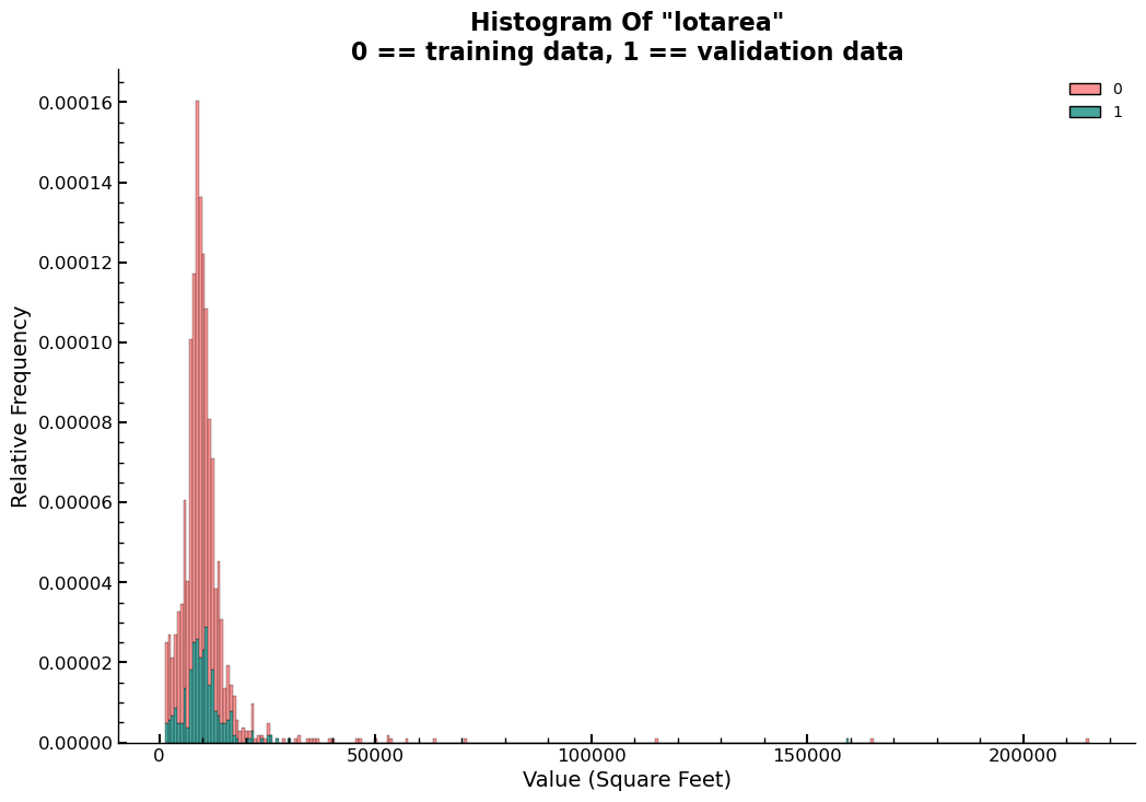
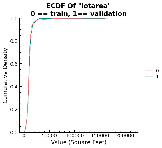
The following code section presents a comprehensive implementation of the feature selection process discussed earlier. The code demonstrates the precise method used to drop the garagearea feature from both the train and validation data while maintaining consistency in the column names for future use. Moreover, the code includes a histogram plot and an ECDF plot of the density of values in lotarea, illustrating a case where there is no apparent difference in the distributions of a variable’s values between the train and validation sets. This visualization is vital in helping professionals identify any issues with the data and emphasizes the need for meticulous feature selection to ensure precise and dependable machine learning models. The code section offers a practical demonstration of the feature selection process and underscores the significance of attention to detail when working with complex data in machine learning projects.

for i in ["xs_final_ext", "valid_xs_final_ext"]:
    pd.to_pickle(i, f"{i}.pkl")

finalcolsdict = {
    "xs_final_ext": xs_final_ext.columns.tolist(),
    "valid_xs_final_ext": valid_xs_final_ext.columns.tolist(),
}

plt.close("all")
fig = plt.figure(figsize=(6,6))
sns.histplot(data=df_comb, x="lotarea", hue=valt,stat='density',multiple='stack',)
plt.title('Histogram Of "lotarea"\n0 == training data, 1 == validation data')
plt.ylabel('Relative Frequency')
plt.xlabel('Value (Square Feet)')
sns.displot(data=df_comb, x="lotarea", hue=valt,kind='ecdf')
plt.title('ECDF Of "lotarea"\n0 == training data, 1 == validation data')
plt.ylabel('Cumulative Density')
plt.xlabel('Value (Square Feet)')
plt.subplots_adjust(top=.9)

ECDF plot is not rendered well, as it is not yet implemented in matplotlib, according to an error message.

Summary

In this article, we explored the process of feature selection in machine learning projects. We discussed the importance of careful feature selection to ensure accurate and reliable machine learning models, and demonstrated how to identify and drop features that may impact model accuracy. We also examined the out-of-domain problem, which can occur when a model is asked to make predictions on data outside the range of what it has seen during training. Through practical examples and visualizations, we emphasized the need for attention to detail when working with complex data, and provided insights into the feature selection process that can help ensure the reliability and accuracy of machine learning models in industry settings. By following these best practices, data professionals can ensure the success of their machine learning projects and build models that are both effective and reliable.

Entire Series:

Advanced Missing Value Analysis in Tabular Data, Part 1
Decision Tree Feature Selection Methodology, Part 2
RandomForestRegressor Performance Analysis, Part 3
Statistical Interpretation of Tabular Data, Part 4
Addressing the Out-of-Domain Problem in Feature Selection, Part 5
Kaggle Challenge Strategy: RandomForestRegressor and Deep Learning, Part 6
Hyperparameter Optimization in Deep Learning for Kaggle, Part 7