Hyperparameter Optimization in Deep Learning for Kaggle, Part 7
Kaggle Submission 2: tabular_learner deep learning estimator optimized using manual hyperparameter optimization. XGBRegressor using RandomizedSearchCV and sampling from continuous parameter distributions.
Series: Kaggle Competition - Deep Dive Tabular Data
Advanced Missing Value Analysis in Tabular Data, Part 1
Decision Tree Feature Selection Methodology, Part 2
RandomForestRegressor Performance Analysis, Part 3
Statistical Interpretation of Tabular Data, Part 4
Addressing the Out-of-Domain Problem in Feature Selection, Part 5
Kaggle Challenge Strategy: RandomForestRegressor and Deep Learning, Part 6
Hyperparameter Optimization in Deep Learning for Kaggle, Part 7
Hyperparameter Optimization in Deep Learning for Kaggle, Part 7
Optimization of tabular_learner
In order to achieve the best possible performance from the tabular_learner
model, a manual hyperparameter optimization routine is applied using the
dataloaders objects created for training and final predictions. Since this
dataset is relatively small, with less than 2000 rows, a 10 core CPU machine is
sufficient for the optimization process.
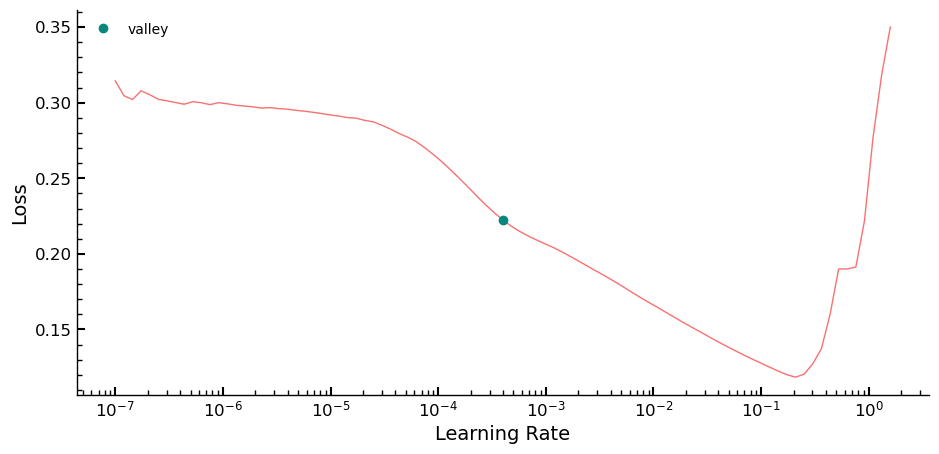
The first step in the optimization routine is to use the lr_find method to
identify the optimal learning rate (lr) value for the model. Given the small
size of the training set, overfitting occurred quickly, and it was found that a
small value for lr worked best in this case. To determine the range of values
for lr, the linspace function was used to test a range of values. Epochs
were tested in increments of 5 between 20 and 40. Early testing showed that this
range produces relatively consistent RMSE values on the validation set, allowing
for a more targeted and efficient hyperparameter search process.
learn.lr_find()
SuggestedLRs(valley=0.0003981071640737355)
linspace_rmse = {"lr": [], "epochs": [], "rmse": []}
preds_targs = {"nn_preds": [], "nn_targs": []}
linspace = [*np.linspace(0.000007, 0.1, 4)]
epochs = [*np.arange(20, 40, 5)]
setups = product(linspace, epochs)
for i in setups:
    linspace_rmse["lr"].append(float(i[0]))
    linspace_rmse["epochs"].append(i[1])
    with learn.no_logging():
        learn.fit(i[1], float(i[0]))
    preds, targs = learn.get_preds()
    preds_targs["nn_preds"].append(preds)
    preds_targs["nn_targs"].append(targs)
    linspace_rmse["rmse"].append(r_mse(preds, targs))
Final values for the tested parameters that result in the lowest RMSE value on the training data are found using the code below.
dfopt = pd.DataFrame(linspace_rmse).sort_values(by="rmse").iloc[:5]
preds_index = dfopt.index[0]
preds = preds_targs["nn_preds"][preds_index]
print(r_mse(preds_targs["nn_preds"][preds_index], preds_targs["nn_targs"][preds_index]))
dfopt
0.132921
| lr | epochs | rmse | |
|---|---|---|---|
| 6 | 0.033338 | 30 | 0.132921 |
| 7 | 0.033338 | 35 | 0.140671 |
| 9 | 0.066669 | 25 | 0.151811 |
| 5 | 0.033338 | 25 | 0.159139 |
| 8 | 0.066669 | 20 | 0.161941 |
Using an ensemble, consisting of the tabular_learner and the optimized
RandomForestRegressor estimator is evaluated below, accounting for the
consistently better predictions of the RandomForestRegressor compared to the
ones of the tabular_learner, the predictions of the RandomForestRegressor
are weighted twice as much as the ones from the tabular_learner.
The general idea is that different types of models have different rows for which their predictions are superior to those of the other models in the ensemble, and therefore an ensemble of models can potentially achieve better predictions over the entire set of rows compared to the predictions of the individual models in the ensemble.
This simple ensemble resulted in the lowest RMSE value recorded so far on the validation set.
preds2, _ = learn.get_preds(dl=tonn_vfs_dl)
rf_preds = m2.predict(x_val_nnt)
ens_preds = (to_np(preds.squeeze()) + 2 * rf_preds) / 3
r_mse(ens_preds, y_val)
0.126166
Optimization of XGBRegressor
The XGBRegressor is a highly competitive tree ensemble-based model that has
demonstrated superior predictive accuracy in numerous Kaggle and other platform
competitions. To achieve the best performance from this model, careful
hyperparameter tuning is required during the fitting process, which should be
complemented with robust cross-validation techniques to prevent overfitting on
the training data.
The hyperparameter optimization procedure is carried out using the parameters specified in the dmlc XGBoost version of the model. For a comprehensive list of parameters and their descriptions, please refer to the dmlc XGBoost Parameter Documentation. The Scikit-Learn API, which can also be found in the documentation (Scikit-Learn XGBoost API Documentation), is utilized in the code below.
To facilitate hyperparameter optimization, we have developed two functions:
RMSE and get_truncated_normal. get_truncated_normal is a custom continuous
distribution derived from the normal distribution, which ensures that none of
its values exceed a specified value range. By adjusting the distribution’s bell
curve shape, the value distribution can be fine-tuned between the upper and
lower limits. It is advisable to use sampling with replacement to prevent the
algorithm from being restricted by a dwindling pool of values to sample from.
Moreover, it is highly recommended to use continuous distributions to sample
from for continuous parameters, as mentioned in the documentation:
If all parameters are presented as a list, sampling without replacement is performed. If at least one parameter is given as a distribution, sampling with replacement is used. It is highly recommended to use continuous distributions for continuous parameters.
RMSE defines a custom scorer metric that can be used by sklearn to evaluate
the estimator’s predictive accuracy during the optimization process. This metric
is also the standard evaluation metric used by Kaggle for final submissions.
The RandomizedSearchCV function from the sklearn library is used for
hyperparameter optimization. This function is a variation of the more general
method called random search. Although it shares some similarities with the
grid search method, it differs in several key aspects.
Compared to grid search, which requires the user to pass an exhaustive set of
values to be tested for each parameter to the algorithm, random search is less
restrictive. It samples from the distributions passed for each parameter, given
by the values of the param_dist dictionary, during each iteration. As a
result, random search can cover a wider range of values for each parameter and
use increments as small as the number of iterations passed allows for sampling.
One of the weaknesses of the grid search procedure is that each hyperparameter can have a large value range for its possible values, such as a continuous value range between $0$ and $1$. This range containing all possible machine numbers between $0$ and $1$ cannot be tested in a grid search, as there are too many values in this range. Additionally, the number of models to build during grid search can become extremely high even for a small subset of hyperparameters, making the process computationally expensive. For example, with $15$ hyperparameters and $40$ possible values for each, using a $5$-fold cross-validation would require building $3000$ models, which takes approximately $34$ minutes with a time of $0.68$ seconds per model on the machine used in this case.
To address these issues, random search is chosen over grid search for
hyperparameter optimization. In this implementation, $1400$ iterations are used,
each with an $8$-fold cross-validation, and enable_categorical=True is passed
to account for the categorical variables. The best estimator is then assigned to
variable best, and the RMSE on the validation set is printed out using
estimator best.
def RMSE(preds_indep_test, dep_test):
    return np.sqrt(mean_squared_error(preds_indep_test, dep_test))

def get_truncated_normal(mean, sd, low, upp):
    return scipy.stats.truncnorm(
        (low - mean) / sd, (upp - mean) / sd, loc=mean, scale=sd
    )

model = XGBRegressor(
    random_state=seed, tree_method="hist", nthread=-1, enable_categorical=True
)

param_dist = {
    "n_estimators": scipy.stats.randint(100, 1000),
    "learning_rate": np.random.random_sample(1000),
    "max_depth": scipy.stats.randint(2, 30),
    "subsample": get_truncated_normal(mean=0.6, sd=0.2, low=0, upp=1),
    "colsample_bylevel": get_truncated_normal(mean=0.6, sd=0.4, low=0, upp=1),
    "colsample_bytree": get_truncated_normal(mean=0.6, sd=0.4, low=0, upp=1),
    "colsample_bynode": np.random.choice(
        np.arange(0.1, 1, 0.1), size=1000, replace=True
    ),
    "lambda": np.random.choice(np.arange(0.1, 1.2, 0.01), size=1000, replace=True),
    "alpha": np.random.choice(np.arange(0.1, 1, 0.04), size=100, replace=True),
    "gamma": scipy.stats.expon.rvs(size=1500),
}
n_iter = 1400
kfold = KFold(n_splits=8)
random_search = RandomizedSearchCV(
    model, param_dist, scoring=None, refit=True, n_jobs=-1, cv=kfold, n_iter=n_iter
)
random_result = random_search.fit(x_nnt, y)
best = random_result.best_estimator_
random_proba = best.predict(x_val_nnt)
val_score = RMSE(random_proba, y_val)
print(f"{val_score} val_score")
0.13291718065738678 val_score
Three Model Ensemble
Ensembling is a widely used technique in machine learning that combines multiple
models to improve the overall predictive performance. One common way to weigh
the predictions of the ensemble members is by assigning equal weights to each
model
An ensemble approach combining tabular_learner, RandomForestRegressor, and
XGBRegressor is implemented to further improve the performance of the model.
Each model is given equal weight in the ensemble, and the results exceed those
achieved by individual models. As a result, this ensemble is used in the final
submission, achieving even higher accuracy than the previously employed
approaches.
ens_preds2 = (to_np(preds.squeeze()) + rf_preds + random_proba) / 3
r_mse(ens_preds2, y_val)
0.124315
Kaggle Submission
The val_pred function takes a dataloader and the three optimized estimators as
inputs and generates predictions using all three models. However, since the RMSE
of the predictions is found to be lowest when only using XGBRegressor and
RandomForestRegressor, these two models are chosen for the final predictions
submitted to Kaggle.
To re-transform the predictions before adding them together and dividing by
three, the exponential function is applied to the predictions of each estimator.
The resulting predictions can then be added to a DataFrame under a new column
SalePrice and exported as a CSV file.
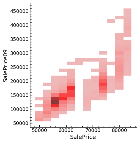
Upon analyzing the results of the Kaggle submission, it was found to be worse
than the best one submitted previously. To identify potential reasons for this,
the predictions of the best submission thus far were imported, and a bivariate
distribution of the dependent variable was plotted and compared. The best
submission corresponds to SalePrice09, and the predictions of this submission are
labeled as SalePrice in the following figures.
def val_pred(tonn_vfs_dl,m2,best,learn):
predsnn, _ = learn.get_preds(dl=tonn_vfs_dl)
predsrf = m2.predict(tonn_vfs_dl.items)
predsxgb = best.predict(tonn_vfs_dl.items)
for i in predsnn,predsrf,predsxgb:
print(type(i),len(i),i.shape)
preds_ens_final = (np.exp(to_np(predsnn.squeeze())) + np.exp(predsrf) + np.exp(predsxgb)) /3
print(preds_ens_final.shape,preds_ens_final[:4])
df_sub=pd.read_csv('../data/sample_submission.csv')
df_sub9=pd.read_csv('../data/submission_9.csv')
df_sub9 = (
df_sub9
.rename_column('SalePrice','SalePrice09')
)
df_sub['SalePrice'] = preds_ens_final
print(df_sub.sample(n=3))
df_sub.to_csv('../portfolio_articles/submission_portfolio.csv',index=False)
df_sub_comp = pd.concat([df_sub[['SalePrice']],df_sub9[['SalePrice09']]],axis=1)
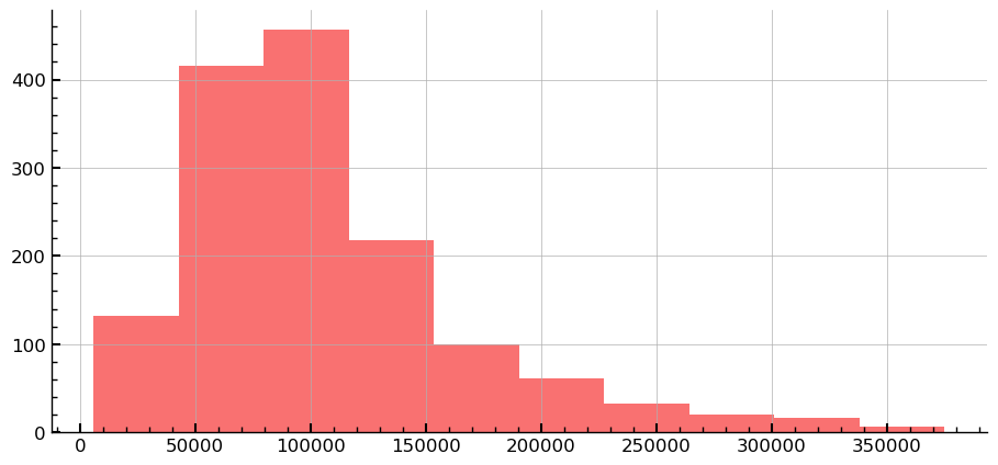
df_sub_comp['diff'] = np.abs(df_sub_comp['SalePrice']-df_sub_comp['SalePrice09'])
df_sub_comp['diff'].hist()
plt.show()
df_sub_comp = (
df_sub_comp
.add_columns(
predsrf=np.exp(predsrf), predsxgb=np.exp(predsxgb)
)
)
return df_sub_comp
df_sub_comp = val_pred(tonn_vfs_dl,m2,best,learn)
print(df_sub_comp.columns)
<class 'torch.Tensor'> 1459 torch.Size([1459, 1])
<class 'numpy.ndarray'> 1459 (1459,)
<class 'numpy.ndarray'> 1459 (1459,)
(1459,) [55746.34455882 59377.90043929 57786.0567984  62267.60988243]
        Id     SalePrice
173   1634  62267.609882
1213  2674  74203.475024
799   2260  61325.784554
Index(['SalePrice', 'SalePrice09', 'diff', 'predsrf', 'predsxgb'], dtype='object')
sns.displot(data=df_sub_comp,x='SalePrice',y='SalePrice09')
plt.show()
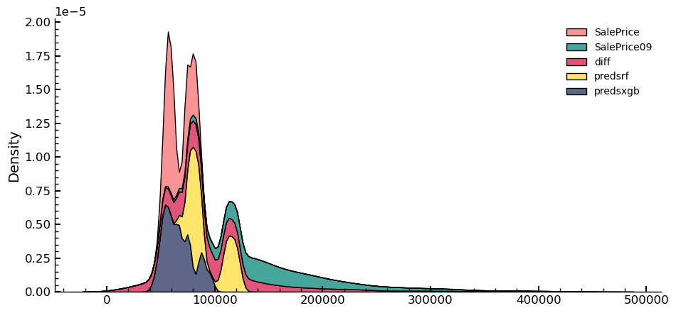
sns.kdeplot(data=df_sub_comp,multiple="stack")
plt.show()
Entire Series:
Advanced Missing Value Analysis in Tabular Data, Part 1
Decision Tree Feature Selection Methodology, Part 2
RandomForestRegressor Performance Analysis, Part 3
Statistical Interpretation of Tabular Data, Part 4
Addressing the Out-of-Domain Problem in Feature Selection, Part 5
Kaggle Challenge Strategy: RandomForestRegressor and Deep Learning, Part 6
Hyperparameter Optimization in Deep Learning for Kaggle, Part 7
© Tobias Klein 2023 · All rights reserved
LinkedIn: https://www.linkedin.com/in/deep-learning-mastery/