Economic Analysis of Hearthstone: Euro to In-Game Currency
Delving into the economic aspects of Hearthstone, this article provides a detailed simulation of in-game currency value, offering insights into the real-world monetary worth of Hearthstone decks.
Economic Analysis of Hearthstone: Euro to In-Game Currency
Hearthstone: Euro To In-Game Currency Conversion

Abstract
This article conducts a comprehensive analysis of the equivalent average dust value (ADV) for a single Hearthstone card pack. It aims to establish a function where Euro expenditure serves as the independent variable, and the equivalent dust value, a universal in-game currency indicative of deck costs, is the dependent variable. The research includes two distinct simulations, with a focus on comparing their runtime and outcomes. Interestingly, the results do not definitively indicate a trend towards a Normal distribution for the ADV. This unexpected outcome is thoroughly examined in light of the central limit theorem and the law of large numbers. The article delves into potential reasons why these classical statistical theories may not align with the observed data, and discusses the broader implications of these deviations on the study’s conclusions.
Research Questions
1. Compare the performance of two different simulation functions written in Python and analyze the results.
- A vectorized function without loops (all numpy)
- A loop based function (some numpy, but no vectorization)
2. What is the ADV per card pack?
3. Show that the distribution of the ADV converges against a normal
distribution $N(\mu_{N},\sigma_{N})$ with \(\mu_{N}\,=\hat{\mu}\) and
\(\sigma_{N}\,=\,\hat{\sigma}\), \(\hat{\mu}\) and \(\hat{\sigma}\) being the
empirical mean and standard deviation from the simulation, as stated by the
central limit theorem.
4. Explain how the Law of Large Numbers applies here.
5. How is the function defined that maps Euro spent to the equivalent dust
value.
Introduction
From the Wikipedia entry:
Hearthstone is a free-to-play online digital collectible card game developed and published by Blizzard Entertainment. Originally subtitled Heroes of Warcraft, Hearthstone builds upon the existing lore of the Warcraft series by using the same elements, characters, and relics. Wikipedia
Hearthstone is a popular trading card game that was released by Activision Blizzard in 2014. In 2017, even before the surge in player base caused by the lockdown during the COVID-19 pandemic, the game was reportedly generating as much as $$40 million a month.
The table shows various statistics regarding the player base of the game Hearthstone. It can be said that according to this table, there are around 4 million monthly players on average. Data originates from https://activeplayer.io/hearthstone/ and is only reproduced here.
Basic Principles of the Game
Format
- Every match of traditional Hearthstone, which is the focus of this article, is a 1 vs. 1 match where two players face each other. Each player has a deck of cards consisting of 30 cards. This article is not concerned with how the actual game works and only explains the details needed for this article. For more detailed information regarding the basic game mechanics, please see this official guide for example.
Deck Of Cards
- Each player has to have at least one deck in order to be able to play.
- A deck is a collection of 30 cards.
- The cost of a deck is equal to the sum of the dust costs of all 30 cards in the deck.
- This assumes that the player has none of the 30 cards in his card collection that make up the deck.
- Depending on the distribution of the rarities of the 30 cards (more on that later), a deck can cost between 4,000 to 18,000 dust on average. There are generally many decks that can be found somewhere between these limits.
- These limits apply to decks that do not have golden cards in them. A deck that contains golden cards costs between 4 to 9 times more than a deck without golden cards.
Ways To Acquire Cards
- There are several ways one can acquire the digital cards necessary to create
a deck.
- Use the in-game currency coins to buy packs of cards, which are gained by completing quests among other in-game activities. This method will be referred to as, by playing the game.
- Buying card packs with real money. There are several bundles on offer at the time of writing this article. They are listed in Table 1. There are special offers from time to time, which will not be evaluated in this article.
- Disenchanting cards see The Universal In-Game Currency that are in one’s collection and that can be disenchanted. Generally, all cards that can be bought by purchasing packs, can also be disenchanted.
| Number of Packs in Bundle | Price (Eur.) | Normalized Price (per pack, rounded) |
|---|---|---|
| 2 | 2.99 | 1.5 |
| 7 | 9.99 | 1.43 |
| 15 | 19.99 | 1.33 |
| 40 | 49.99 | 1.25 |
The Universal In-Game Currency
- Dust is the universal currency in the game for calculating the actual cost
associated with acquiring/crafting (creating) any card and ultimately deck.
- There are 4 classes of cards and each class has a golden variant. They
are:
- common and golden common
- rare and golden rare
- epic and golden epic
- legendary and golden legendary
- The Golden variants are rarer compared to their non-golden counterparts. They cost multiple times more dust to create compared to their non-golden counterparts, but also give more dust when disenchanted.
- Disenchanting means deleting the card from one’s collection in exchange for dust. See table 2, for the exact dust values for each rarity class.
- There are 4 classes of cards and each class has a golden variant. They
are:
A Pack Of Cards
- Each pack of cards has 5 cards. Each card can be of any rarity (See Table 2 for the names of the classes) in general. There is one exception to this, if 4 out of the 5 cards are of the lowest rarity class (Common). In this case, the 5th card will be at least of Rare quality, the second lowest rarity class in terms of drop chance and dust value. This mechanism is not relevant for this simulation however, since only complete sets of drop chances that cover all rarity classes are considered. More on drop chances in the following.
The Odds
Hearthstone and many other computer games rely on a loot box system for monetization. Its aim is to make the player either spend time earning coins by playing the game or/and money to acquire new cards by buying packs of cards. The loot box system relies on in-game items that give the player loot, cards from card packs in this instance. The set of probabilities (draw chances) associated with how likely it is to draw a card of a certain rarity class when opening a pack of cards (see table 2 for exact values), does not have to be disclosed by Blizzard. There is only China as of now that demands what seems like a partial disclosure of the drop chances for any video game company that wants to enter the Chinese market with their video game. See statement below for more.
What We Know
Original Statement (Chinese)
关于《炉石传说》卡牌包抽取概率的公示方式调整公告 发布日期:2018-08-02 《炉石传说》现将抽取卡牌的概率公示方式进行调整,具体如下: 《炉石传说》卡牌包共有5张卡牌,包含4种不同品质(普通、稀有、史诗、传说) 稀有卡牌 每个炉石卡牌包,至少能获得一张稀有或更高品质的卡牌。即100%的卡牌包可至少开出稀有或更高品质(史诗、传说)的卡牌。 史诗卡牌 约20%的卡牌包可开出史诗品质卡牌。 传说卡牌 约5%的卡牌包可开出传说品质卡牌。 备注:
- 每个账号首次打开10包同一种类卡牌包(如经典、女巫森林、砰砰计划等),必定可开出传说品质卡牌。
- 本次公告调整仅涉及概率公示方式的调整。《炉石传说》卡牌包的实际抽取概率并未发生改变。
English Translation
Announcement on the adjustment of the disclosure method of the card pack extraction probability of “Hearthstone Legend Release date: 2018-08-02 The Legend of Hearthstone is now adjusting the public announcement method of the probability of card extraction, as follows. Hearthstone Legend card pack has 5 cards, including 4 different qualities (common, rare, epic, legend) Rare cards Each Hearthstone card pack, you can get at least one rare or higher quality card. That is, 100% of the packs can open at least rare or higher quality (epic, legendary) cards. Epic Cards About 20% of card packs open Epic quality cards. Legendary Cards Approximately 5% of the packs will yield Legendary quality cards. Remark.
- The first time each account opens 10 packs of the same kind of cards (such as Classic, Witch’s Wood, Bang Bang Project, etc.), it will definitely open Legendary quality cards.
- This announcement only involves the adjustment of the probability announcement method. The actual probability of drawing cards from The Legend of Hearthstone packs has not changed.
The statement from Blizzard reveals only some of the drop chances associated with opening card packs. What can be gained from the statement is the following:
-
At least one card in any pack will be of class rare or higher.
This fact is not of relevance for this case study, as discussed in section ‘Basic Principles of the Game, Bullet Point 5.’)
-
Cards of the class epic have a 20% drop chance.
This is valuable, since it gives a presumably accurate drop chance for epic cards. It is not a number that comes from empirical testing, but from the creator of the draw mechanism itself. It is therefore used in the following.
-
Legendary cards have a drop chance of 5%.
As with the drop chance for epic cards, this number is used in the following. See epic card drop chance for the reasoning.
Calculation of Odds
Sources
With the drop chances for epic and legendary cards from the afore mentioned Blizzard statement and various empirical studies where people opened packs and counted the cards they had opened during the study (source), as references, the drop rates were calculated as follows.
Sorting By Rarity
- All empirical studies showed that the drop chances follow an order. From least to most likely, for all classes: 1. Golden Legendary 2. Golden Epic 3. Golden Rare 4. Golden Common 5. Legendary 6. Epic 7. Rare 8. Common
Limitations
It must be noted that all empirical studies were conducted before 2018. Blizzard’s statement is the most recent information, and it is presumed that It is valid for sales made outside of China as well. Empirical experiments conducted on the distribution of the rarity classes mentioned in the Blizzard statement did not match those that Blizzard disclosed in the statement above, as well as because the sum of probabilities for all classes wasn’t exactly 1.0. So some adjustments had to be made, to arrive at a set of probabilities that is consistent with Blizzard disclosed numbers where the sum of probabilities is exactly 1.0 as well.
Final Odds
The final values for the drop chances used, come from the sources mentioned earlier and from testing different sets of drop chances, in order to rule out sets that either violate the order outlined or don’t sum up to exactly 1 or violate the information given by Blizzard. The final, correct set of drop chances remains unknown, but using the simulation approach outlined in the following, any valid set can be tested and its results analyzed. The drop chances can be found in table 2.
Table 2 The columns of Table 2 show, from left to right: All card classes in the ‘Class’ column. The ‘Draw Chance’ column gives the drop chances for each class and ‘Dust Value’ gives the amount of dust that disenchanting the respective class gives.
| Class | Draw Chance | Dust Value |
|---|---|---|
| golden legendary | 0.0007 | 1600 |
| golden epic | 0.0023 | 400 |
| golden rare | 0.0133 | 100 |
| golden common | 0.0137 | 50 |
| legendary | 0.05 | 400 |
| epic | 0.2 | 100 |
| rare | 0.25 | 20 |
| common | 0.47 | 5 |
Money To Dust Value Function
With \(m\) the money spent, \(n\) the number of packs bought. \(n\) can be any linear combination of the number of packs available, as shown in Table 1. \(p\) is the price for \(n\) packs. \(\mathit{ADV}\) is the dust average per pack from the simulation.
\[\def\lf{\left\lfloor} \def\rf{\right\rfloor} f(m,n,p,\mathit{ADV})= \lf \frac{m}{p} \rf \cdot \mathit{ADV} \cdot n\]The result is a linear function, with a bias of 0 and gradient larger 1 for all possible values of \(n\). The steepest gradient is found for multiples of the largest card pack bundle with 40 packs in each bundle.
Simulation Of Dusting Hearthstone Cards
The term ‘dusting’ here refers to the act of disenchanting hearthstone cards. During the process of dusting a card, the card becomes permanently deleted from one’s card collection. In return, one gets the dust value that the card is worth. Please refer to Table 2 for further details.
Imports
import matplotlib.pyplot as plt
import numpy as np
from numpy.random import RandomState, seed
import pandas as pd
import time

plt.style.use("science")
from statsmodels.distributions.empirical_distribution import ECDF
from scipy import stats

seed(42)
plt.ion()
plt.close("all")
Numpy Vectorization Implementation (NVI)
Inputs
The following is a much better way to define the numbers needed for the
simulation than is used in the original loop based implementation, described
next. With a dictionary, the relevant input values are defined for the
simulations. trials specifies the number of trials to simulate, each with the
number of packs packs. probs gives the draw chances for each class. cats
is used to transform the string rarity classes into integer ones. dust gives
the dust value for each rarity class.
# order draw_chances values to create intervals for drawing mechanism
inputs = {
    "trials": np.int_(1e5),
    "packs": np.int_(40),
    "probs": {
        "glegendary": np.double(0.0007),
        "gepic": np.double(0.0023),
        "grare": np.double(0.0133),
        "gcommon": np.double(0.0137),
        "legendary": np.double(0.05),
        "epic": np.double(0.2),
        "rare": np.double(0.25),
        "common": np.double(0.47),
    },
    "cats": {
        "glegendary": 7,
        "gepic": 5,
        "grare": 3,
        "gcommon": 1,
        "legendary": 6,
        "epic": 4,
        "rare": 2,
        "common": 0,
    },
    "dust": {
        "glegendary": np.int_(1600),
        "gepic": np.int_(400),
        "grare": np.int_(100),
        "gcommon": np.int_(50),
        "legendary": np.int_(400),
        "epic": np.int_(100),
        "rare": np.int_(20),
        "common": np.int_(5),
    },
}
NVI Function Definition
Using the default numpy rng generator, with output values from dust,
probabilities probs and size the product of trials, packs and 5. There are
5 cards in each card pack. Using cards.reshape(trials,packs,5) to create a
ndarray with suitable dimensions, the ADV over each trial is calculated and
returned along with the standard deviation for the distribution of the ADV.
def sim_rc(
    packs=inputs["packs"],
    trials=inputs["trials"],
    probs=[*inputs["probs"].values()],
    dust=[*inputs["dust"].values()],
):
    rng = np.random.default_rng()
    s = np.product([packs, trials, 5])
    cards = np.array(rng.choice(a=dust, size=s, p=probs))
    sima = cards.reshape(trials, packs, 5)
    dust_avg_t = [np.sum(tt) / packs for tt in sima]
    dust_avg = np.mean(dust_avg_t)
    dust_std = np.std(dust_avg_t)
    return dust_avg_t, dust_std, dust_avg
NVI Call Function
start_np = time.time()
np_mu_trial, np_std, np_mu = sim_rc()
total_time_np = time.time() - start_np
print(
f'The system time duration, total cards generated for the NVI is: {total_time_np}, {inputs["packs"]*inputs["trials"]*5:,}'
)
fig, ax = plt.subplots(1, 1, figsize=(12, 10))
ax = plt.subplot(111)
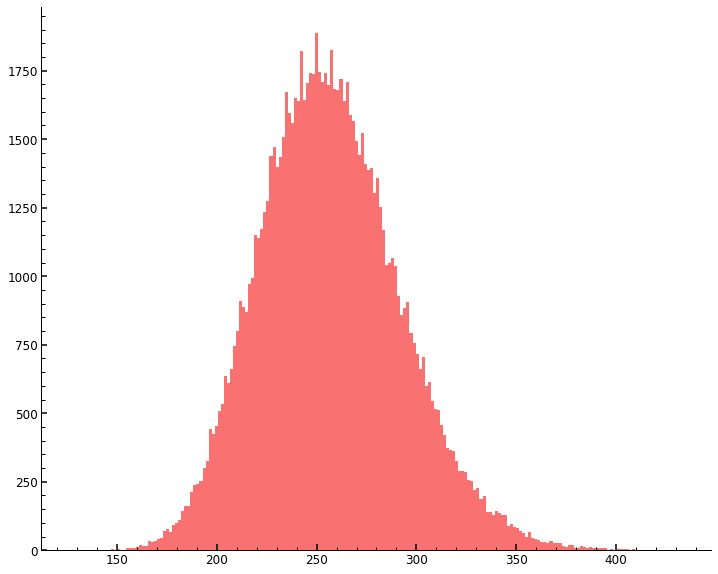
ax.hist(np_mu_trial, density=False, bins=200, label="histogram", alpha=1)
plt.show()
The system time duration, total cards generated for the NVI is: 0.8454718589782715, 20,000,000
print(
    f"The sorted drop chances for the classes are: {[*zip([*inputs['cats'].values()],[*inputs['probs'].values()])]}"
)
print(f"The sum of the sorted drop chances is: {sum([*inputs['probs'].values()]):.4f}")
The sorted drop chances for the classes are: [(7, 0.0007), (5, 0.0023), (3, 0.0133), (1, 0.0137), (6, 0.05), (4, 0.2), (2, 0.25), (0, 0.47)]
The sum of the sorted drop chances is: 1.0000
Loop Implementation (LI)
This implementation should not be used, it is much slower than the NVI using only numpy vectorization. It is only included for comparison and learning purposes.
Motivation Optional
This is the first implementation I wrote back in 2019, when I was still actively
playing Hearthstone and wanted to know how much money I had to spend (on
average), in order to be able to craft a ‘Golden Zephrys the Great’ (Cost: 3200
dust). The card is special, as it uses machine learning, to understand what the
best three cards are for the player at the time of the card being played. It
then offers the player these three cards and plays the one chosen. In Blizzard’s
words, the model had to be changed, so its predictions were not as refined and
‘imbalanced’ anymore.

In short, they nerfed the card soon after its addition to the game. Interestingly, the machine learning model behind this mechanic was sophisticated enough that even Blizzard said that they could not always forecast what the three chosen cards would be, as the models predictions in the form of the three ‘perfect’ cards presented to the player were the result of some sort of ‘black box’ type of model. My guess is that it is a deep learning model.
Anyway, after this brief motivation of why I embarked on the project of simulating the ‘opening of hearthstone card packs’ in the first place, I present the original loop implementation.
LI Inputs
A discrete distribution with intervals for each rarity class on the domain \([0,1]\) is used. The intervals are constructed, so that the area of each interval is equal to the respective drop chance of the rarity class it represents.
Each interval is defined by the lower and upper limit of the half open interval
between _l and _h (\((\,\_l,\_h]\,\)) for all rarity classes, like:
gl_l=goldenlegendary_low and gl_h=goldenlegendary_high for example.
Starting by zero, the intervals are added to the upper limit of the previous
rarity class from the class with the lowest draw chance up to the class with the
highest. The sum of the intervals must equal exactly 1 to be a valid set of
probabilities.
# creating interval borders: '_l'/'_h' stand for the low end and high end of the interval respectively.
gl_l = 0.0
gl_h = 0.0007
ge_l = gl_h
ge_h = gl_h + 0.0023
gr_l = ge_h
gr_h = ge_h + 0.0133
gc_l = gr_h
gc_h = gr_h + 0.0137
l_l = gc_h
l_h = gc_h + 0.05
e_l = l_h
e_h = l_h + 0.2
r_l = e_h
r_h = e_h + 0.25
c_l = r_h
c_h = r_h + 0.47

print(
    f"The probability of a common class card to be drawn is {np.round(1-c_l,decimals=2)}"
)

# Defining rarity colors by integer numbers
rarity_dict = {
    "common": 0,
    "golden_common": 1,
    "rare": 2,
    "golden_rare": 3,
    "epic": 4,
    "golden_epic": 5,
    "legendary": 6,
    "golden_legendary": 7,
}
The probability of a common class card to be drawn is 0.47
LI Function Definition
A numpy function is used to generate random numbers from a uniform distribution
on the domain \([0,1)\). Half open intervals used for the probability account
for the domain of the numpy function used. The product of packs per trial, trial
and 5 (there are 5 cards in each pack) gives the total number of random numbers
it generates. np.nditer is used to create an iteratee over which then is
iterated. The outer most loop over onet loops over each trial. With the next one
looping over each pack opened in each trial (draws_onet). The inner most loop
then loops over the opening of the five cards in every pack (rows[:]).
Each random number that represents one drawn card in a pack of five cards,
is evaluated as to which of the intervals it lies within and the corresponding
rarity class and dust value is appended to a list. There are lists for each
loop and lists all_packs, all_dust hold these values for the entire
simulation.
def hs_sim(packs, trials):
    """Function that simulates opening Hearthstone card packs. Each card drawn
    is logged, including its rarity class and dust value."""

    print(f"Simulating {trials:,} trials, each with {packs} card packs")
    all_draws = np.random.uniform(size=packs * trials * 5)
    all_draws = all_draws.reshape(trials, packs, 5)
    # create iterator over trials axis.
    onet = np.nditer(np.arange(0, trials, 1))
    all_packs, all_dust = [], []
    # loop over each trial.
    for i in onet:
        # Only keep i-th trial index value and all index values for 2nd,3rd
        # axes.
        draws_onet = all_draws[i]
        # reset trial stats at start of every trial.
        dust_onet, cards_onet = [], []
        # loop over each pack in the trial with all 5 column values in each row.
        for row in draws_onet:
            # reset values for pack contents after 5 cards have been opened.
            # 5 cards per pack to open.
            cards_onep, dust_onep = [], []
            # For each opened card, identify it and add corresponding values for
            # type and dust value to cards_onep and dust_onep.
            for draw_result in row[:]:
                card_single, dust_single = -999, -900
                # 1 golden legendary
                if draw_result <= gl_h:
                    card_single, dust_single = 7, 1600
                # 2 golden epic
                elif ge_l < draw_result <= ge_h:
                    card_single, dust_single = 5, 400
                # 3 golden rare
                elif gr_l < draw_result <= gr_h:
                    card_single, dust_single = 3, 100
                # 4 golden common
                elif gc_l < draw_result <= gc_h:
                    card_single, dust_single = 1, 50
                # 5 legendary
                elif l_l < draw_result <= l_h:
                    card_single, dust_single = 6, 400
                # 6 epic
                elif e_l < draw_result <= e_h:
                    card_single, dust_single = 4, 100
                # 7 rare
                elif r_l < draw_result <= r_h:
                    card_single, dust_single = 2, 20
                # 8 common
                elif c_l < draw_result <= c_h:
                    card_single, dust_single = 0, 5
                # append dust value of card in pack.
                dust_onep.append(dust_single)
                # append card category of card in pack.
                cards_onep.append(card_single)
            # at the end of each pack opening append all values in dust_onep to
            # dust_onet.
            dust_onet.append(dust_onep)
            # at the end of each pack opening append all values in cards_onep to
            # cards_onet.
            cards_onet.append(cards_onep)
        # at the end of each trial append all values in dust_onet to
        # all_dust.
        all_dust.append(dust_onet)
        # at the end of each trial append all values in cards_onet to
        # all_packs.
        all_packs.append(cards_onet)
    # create ndarrays, with two dimensions (trials,packs*5)
    all_packs = np.array(all_packs).reshape(trials, packs * 5)
    all_dust = np.array(all_dust).reshape(trials, packs * 5)
    # return the two ndarrays
    return all_packs, all_dust
LI Call Function
The LI function is given the same inputs as the NVI and its duration is logged as well.
mm = (inputs["packs"], inputs["trials"])
packs, trials = mm[0], mm[1]

start_for_loop = time.time()
a1, a2 = hs_sim(packs, trials)
total_time_for_loop = time.time() - start_for_loop
print(
    f'The system time duration, total cards generated for the LI is: {total_time_for_loop}, {inputs["packs"]*inputs["trials"]*5:,}'
)
Simulating 100,000 trials, each with 40 card packs
The system time duration, total cards generated for the LI is: 22.610981941223145, 20,000,000
Research Question 1 - Conclusion
- Compare the performance of two different simulation functions written in Python and analyze the results.
- A vectorized function without loops (all numpy)
- A loop based function (some numpy, but no vectorization)
Elapsed Time
The difference in elapsed time between the two functions is enormous. Given that this is the actual system time, the time elapsed in executing each implementation can be influenced by the system load on the local machine. There may be a difference in results from one execution to another. The scalar value \(m\) that gives the following relationship between the times for the implementations \(\mathit{LI}_{t}\,=\,m \mathit{NVI}_{t}\) tends to fall within the interval \(m \in \mathbb{R} \cap [25,28]\)
The value of \(m\) with respect to the most recent execution is printed below.
m = total_time_for_loop / total_time_np
print(f"The scalar using the most recent executions is: {m}")
The scalar using the most recent executions is: 26.743624522935473
Simulation Size
It takes the LI ~23 seconds to simulate the drawing of 20,000,000 cards. Given the fact that the NVI always outperforms the LI, it is the NVI that should be considered when simulating large numbers of pack openings.
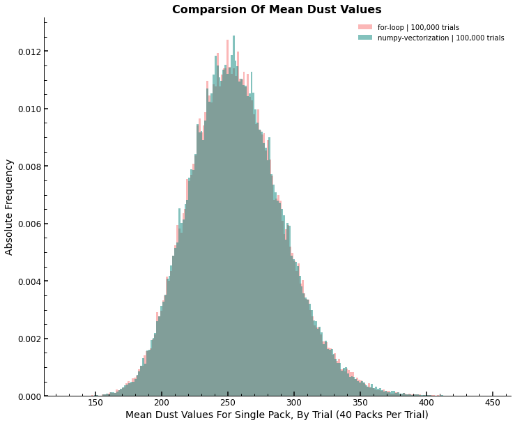
ADV Value And Distribution Comparison
The final ADV value over all trials is close to the same for both. Not only is this true for the ADV value, but also for the PDFs of the ADV per trial. See the histogram below for a comparison of the distributions.
dust_avg_t = [np.sum(tt) / packs for tt in a2]
li_std = np.std(dust_avg_t)
plt.close("all")
fig, ax = plt.subplots(1, 1, figsize=(12, 10))
ax = plt.subplot(111)
ax.hist(
    np_mu_trial,
    density=True,
    bins=200,
    label=f"for-loop | {inputs['trials']:,} trials",
    alpha=0.5,
)
ax.hist(
    dust_avg_t,
    density=True,
    bins=200,
    label=f"numpy-vectorization | {inputs['trials']:,} trials",
    alpha=0.5,
)
ax.set_title(f"Comparsion Of Mean Dust Values")
ax.set_xlabel(
    f"Mean Dust Values For Single Pack, By Trial ({inputs['packs']} Packs Per Trial)"
)
ax.set_ylabel("Absolute Frequency")
ax.legend(loc="best")
plt.show()
Research Question 2 - Conclusion
2. What is the ADV per card pack?
Empirical results for the mean and standard deviation of \(ADV_{trial}\) using 40 packs per trial and 100,000 trials are in dust per card pack:
\[\begin{align*} \hat{\mu}(ADV_{trial}) &= \{\,\,x \in \mathbb{R}\quad |\quad 256 \,\le \, x \, \le \, 258\,\,\}\\ \hat{\sigma}(ADV_{trial}) &= \{\,\,x \in \mathbb{R}\quad |\quad 34 \,\le \, x \,\le 36 \,\,\} \end{align*}\]print(
f"LI - Average dust per trial of the simulation (first five trials with {inputs['packs']} each):\n {dust_avg_t[:5]}"
)
dust_avg_all_trials = np.mean(dust_avg_t)
print()
print(
f"LI - ADV and standard deviation of ADV over all trials in the simulation: {dust_avg_all_trials}, {li_std}"
)
print(
f"NVI - ADV and standard deviation of ADV over all trials in the simulation: {np_mu}, {np_std}"
)
LI - Average dust per trial of the simulation (first five trials with 40 each):
 [282.75, 244.0, 248.875, 242.625, 257.0]

LI - ADV and standard deviation of ADV over all trials in the simulation: 257.0840275, 34.91854175261681
NVI - ADV and standard deviation of ADV over all trials in the simulation: 256.94153875, 35.060196821873355
Further documentation of simulation results. Unique dust values and their respective absolute frequencies over the entire simulation, ordered by unique card categories and indexed with string names of each card category.
un, freq = np.unique(a2, return_counts=True)
keys = [
    "golden_legendary",
    "legendary_golden-epic",
    "epic_golden-rare",
    "golden_common",
    "rare",
    "common",
]
dfu = pd.concat(
    [pd.Series(un), pd.Series(freq)],
    axis=1,
).sort_values(by=0, ascending=False)
dfu.columns = ["unique_dust_categories", "abs_frequency"]
dfu.index = keys
dfu
| unique_dust_categories | abs_frequency | |
|---|---|---|
| golden_legendary | 1600 | 14092 |
| legendary_golden-epic | 400 | 1046900 |
| epic_golden-rare | 100 | 4263543 |
| golden_common | 50 | 273122 |
| rare | 20 | 5000453 |
| common | 5 | 9401890 |
Research Question 3 - Conclusion
Show that the distribution of the Average Dust Value (ADV) converges towards a normal distribution $N(\mu_{N}, \sigma_{N})$ where $\mu_{N} = \hat{\mu}$ and $\sigma_{N} = \hat{\sigma}$, with $\hat{\mu}$ and $\hat{\sigma}$ representing the empirical mean and standard deviation from the simulation. This observation aligns with the predictions of the central limit theorem.
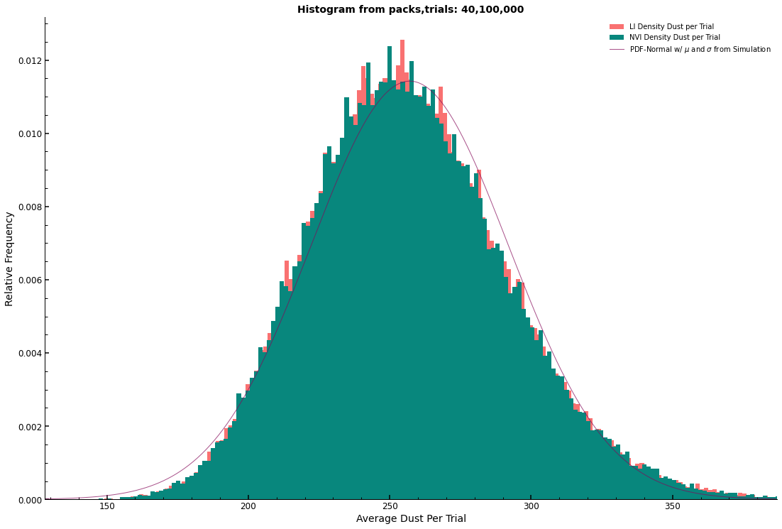
The histogram represents the relative frequency of dust means per trial across the simulation series. It reveals that smaller sample sizes and fewer packs per trial yield distributions less representative of a normal distribution. Conversely, the simulation with 40 packs per trial and 100,000 trials, which is the maximum purchasable quantity at the time of writing, closely approximates a normal distribution with equivalent mean and standard deviation.
According to the Central Limit Theorem (CLT), as sample sizes increase, the sample means should distribute normally, converging on the population mean and standard deviation. In the largest simulation run on a local M1 chip-based Apple machine, 100,000 trials consisted of 40 packs with 5 cards each, totaling 20,000,000 cards. The resulting Probability Density Function (PDF) of the ADV approximates that of a normal distribution with matching mean and standard deviation.
Below, the empirical PDFs from the simulations are juxtaposed against the normal distribution’s PDF. The fit’s precision is not definitive, but the bell-shaped curve is consistent across all three PDFs. The normal distribution employs the simulation’s mean and standard deviation.
# Given simulation data
mu: float = dust_avg_all_trials  # Empirical mean
li_std: float = np.std(dust_avg_t)  # Empirical standard deviation
packs: int = 40
trials: int = 100_000

# Normal distribution range setup
dist: norm = stats.norm(mu, li_std)
low_end: int = int(np.ceil(dist.ppf(0.0001)))
high_end: int = int(np.ceil(dist.ppf(0.9999)))
x_vals: np.ndarray = np.arange(low_end, high_end, 0.5)
y_vals: np.ndarray = dist.pdf(x_vals)

# Plotting the histogram and PDF
fig, ax = plt.subplots(figsize=(18.5, 12.5))
plt.title(f"Histogram from packs,trials: {packs}, {trials:,}", fontsize=14)
ax.hist(dust_avg_t, density=True, bins=200, label="LI Density Dust per Trial")
ax.hist(np_mu_trial, density=True, bins=200, label="NVI Density Dust per Trial")
ax.plot(x_vals, y_vals, color="#850859", alpha=0.7, label="PDF-Normal with μ and σ from Simulation")
ax.set_ylabel("Relative Frequency")
ax.set_xlabel("Average Dust Per Trial")
ax.set_xlim(low_end, high_end)
ax.legend(loc="best", fontsize=10)
plt.show()

print(f"The current mu, sigma have values {mu} and {li_std} respectively.")
The current mu, sigma have values 257.0840275 and 34.91854175261681 respectively.
The ECDF plots provide a visual comparison between the empirical distributions from the simulations and the theoretical CDF of the normal distribution, highlighting the differences.
# create the ECDF plot for the average dust per trial Random Variable
ecdf = ECDF(dust_avg_t)
ecdf_np = ECDF(np_mu_trial)
# The first value in ecdf.x is -inf, which pyplot does not like.
# So the first value in ecdf.x and ecdf.y is dropped to keep their lengths the same.
ecdf.x = ecdf.x[1:]
ecdf.y = ecdf.y[1:]
ecdf_np.x = ecdf_np.x[1:]
ecdf_np.y = ecdf_np.y[1:]

# using mu and sigma from above as parameters for the theoretical distribution
dist2 = norm.rvs(mu, li_std, 20000000)
dist2s = np.sort(dist2)
ecdf_n = np.arange(1, len(dist2s) + 1) / len(dist2s)
plt.close("all")
fig, ax = plt.subplots(1, 1, figsize=(12, 10), constrained_layout=True)
plt.title(
    f"Theoretical CDF from μ, σ from packs,trials:\n{packs},{trials:,} and ECDF ",
    fontsize=14,
)
ax.plot(dist2s, ecdf_n, color="blue", alpha=0.8, label="Theoretical CDF")
ax.plot(ecdf.x, ecdf.y, color="#FC5A50", alpha=0.8, label="ECDF for-loop")
ax.plot(ecdf_np.x, ecdf_np.y, color="#08877d", alpha=0.8, label="ECDF Numpy")
ax.set_ylabel("CDF")
ax.set_xlabel("Average Dust per Trial")
ax.set_xlim(130, 410)
plt.legend(loc="best")
plt.show()

Given the distinctions between the ECDF and theoretical CDF, the question remains whether the sample means from the simulation are normally distributed or not. To complement the visual analysis done so far, we perform the following statistical tests:
def shapiro_wilk_test(np_mu_trial):
    stat, p_value = stats.shapiro(np_mu_trial)
    print(f'Shapiro-Wilk Test: Statistics={stat:.3f}, p-value={p_value:.3f}\n')
    if p_value > 0.05:
        print('\tSample looks Gaussian (fail to reject H0)\n')
    else:
        print('\tSample does not look Gaussian (reject H0)\n')


def kolmogorov_smirnov_test(data):
    # Compare with a normal distribution with the same mean and std as the data
    norm_dist = stats.norm(loc=np.mean(data), scale=np.std(data))
    stat, p_value = stats.kstest(data, norm_dist.cdf)
    print(f'Kolmogorov-Smirnov Test: Statistics={stat:.3f}, p-value={p_value:.3f}\n')
    if p_value > 0.05:
        print('\tSample looks Gaussian (fail to reject H0)\n')
    else:
        print('\tSample does not look Gaussian (reject H0)\n')


def anderson_darling_test(data):
    result = stats.anderson(data)
    print('Anderson-Darling Test:\n')
    print(f'\tStatistic: {result.statistic:.3f}')
    for i in range(len(result.critical_values)):
        sl, cv = result.significance_level[i], result.critical_values[i]
        if result.statistic < cv:
            print(f'\tAt the significance level {sl}, data looks Gaussian (fail to reject H0).')
        else:
            print(f'\tAt the significance level {sl}, data does not look Gaussian (reject H0).')


# Run tests
shapiro_wilk_test(np_mu_trial)
kolmogorov_smirnov_test(np_mu_trial)
anderson_darling_test(np_mu_trial)
Shapiro-Wilk Test: Statistics=0.994, p-value=0.000

	Sample does not look Gaussian (reject H0)

Kolmogorov-Smirnov Test: Statistics=0.023, p-value=0.000

	Sample does not look Gaussian (reject H0)

Anderson-Darling Test:

	Statistic: 115.166
	At the significance level 15.0, data does not look Gaussian (reject H0).
	At the significance level 10.0, data does not look Gaussian (reject H0).
	At the significance level 5.0, data does not look Gaussian (reject H0).
	At the significance level 2.5, data does not look Gaussian (reject H0).
	At the significance level 1.0, data does not look Gaussian (reject H0).


scipy/stats/_morestats.py:1800: UserWarning: p-value may not be accurate for N > 5000.
  warnings.warn("p-value may not be accurate for N > 5000.")
The provided distribution delineates the probabilities for various outcomes, such as ‘legendary’, ‘epic’, ‘rare’, and ‘common’, within each individual draw. This discrete probability distribution forms the basis for the simulation, where each of the five draws within a pack is presumed independent and adheres to the specified distribution, thus constituting the aggregate distribution of these draws.
Notably, the individual draw distribution does not exhibit normality-evidenced by the asymmetrical probabilities heavily biased towards ‘common’ outcomes. Nonetheless, the CLT assures that the distribution of sample means will approximate a normal distribution as the sample size burgeons, provided the draws are independent and identically distributed (i.i.d.) with a finite variance.
In the simulations under discussion, each trial encompasses 40 packs with 5 cards each, translating to each sample mean being derived from 200 individual draws. According to the CLT, as the number of draws (n) escalates, the sampling distribution of the sample mean should converge towards a normal distribution, irrespective of the initial distribution’s shape, assuming the i.i.d. condition and a finite variance are satisfied.
The probability distribution at hand implies a finite variance, hence the CLT is applicable. Yet, the skewness and kurtosis intrinsic to the original distribution may slow the convergence of the sample mean towards normality. The pronounced skewness-manifest in the high probability of ‘common’ outcomes-suggests that a greater number of draws might be necessary for the sampling distribution of the sample mean to present as normally distributed.
Statistical tests rejecting normality in this context may stem from multiple factors:
-
Skewness of the Original Distribution: The marked skewness indicates that 200 draws may not suffice for the distribution of sample means to manifest normality as posited by the CLT. See “Skewed Dust Distribution” plot below.
-
Sensitivity of Normality Tests: Given an extensive sample size, tests for normality are prone to heightened sensitivity, flagging minor deviations from normality that might be statistically, but not practically, significant.
-
Interdependence of Draws: Should there be a dependence between draws, such as a ‘common’ draw influencing subsequent probabilities within the same pack, this would contravene the i.i.d. premise essential for the CLT.
Acknowledging these nuances, it remains plausible for the sample mean to approximate a normal distribution. However, the skewness of the underlying distribution may necessitate a sample size exceeding 200 draws for such normality to be evident. Furthermore, the large sample size may amplify the normality tests’ sensitivity. In scenarios where normality tests are imperative, such as in hypothesis testing or confidence interval construction, alternative approaches like bootstrap methods or other non-parametric resampling techniques might be employed, which do not hinge on the presumption of normality.
def probs_by_dust_value(
    cats: Dict[str, int], probs: Dict[str, float], dust: Dict[str, int]
) -> Dict[List[str], List[float]]:
    """
    Merges categories with the same dust value and sums their probabilities.

    Args:
    cats (Dict[str, int]): Dictionary of categories and their corresponding identifiers.
    probs (Dict[str, float]): Dictionary of categories and their probabilities.
    dust (Dict[str, int]): Dictionary of categories and their dust values.

    Returns:
    Tuple[List[str], List[float]]: Merged categories and their corresponding summed probabilities.
    """
    dust_to_cats = {}
    for cat in cats:
        dust_val = dust[cat]
        if dust_val not in dust_to_cats:
            dust_to_cats[dust_val] = (str(dust_val), probs[cat])
        else:
            existing_cat, existing_prob = dust_to_cats[dust_val]
            dust_to_cats[dust_val] = (existing_cat, existing_prob + probs[cat])

    categories_merged = [val[0] for val in dust_to_cats.values()]
    probs_merged = [val[1] for val in dust_to_cats.values()]
    dict_merged = dict(zip(categories_merged, probs_merged))
    sorted_dict = dict(sorted(dict_merged.items(), key=lambda item: item[1]))

    return sorted_dict


cat_probs_merged = probs_by_dust_value(inputs["cats"], inputs["probs"], inputs["dust"])
categories_merged, probs_merged = cat_probs_merged.keys(), cat_probs_merged.values()

plt.close("all")
fig, ax = plt.subplots(1, 1, figsize=(8, 6))

categories = categories_merged
y_vals = probs_merged
ax.bar(
    categories, y_vals, label="Distribution of Categories", color="#08877d", alpha=0.8
)
ax.set_title("Skewed Dust Distribution")
ax.set_ylabel("Probability of Drawing (Difference in Magnitude)")
ax.set_xlabel("Unique Dust Categories")
ax.set_xticklabels(categories, rotation=45)
ax.set_yscale('log')
plt.show()

Research Question 4 - Conclusion
4. Explain how the Law of Large Numbers applies here.
By the Law of Large Numbers the sample mean will converge against the population mean, as the sample size tends to infinity. In a simulation, the number of samples generated should be as large as possible. This is to ensure that the empirical mean approximates the population mean as closely as possible.
Research Question 5 - Conclusion
5. How is the function defined that maps Euro spent to the equivalent dust value?
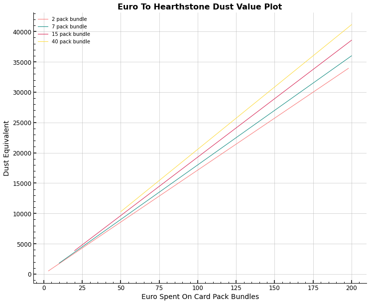
For each of the available card pack bundles, (2, 7, 15, 40 packs per bundle that is) the function mapping Euro spent on card packs to the respective dust equivalent has different parameter values. The plot shows the line plots for all available bundles and compares their linear Euro to dust functions. The dust equivalent, as a ratio of Euro spent to expected dust is lowest for the smallest bundle containing 2 card packs for 3 Euro and steadily increases up to the largest bundle of 40 card packs for 50 Euro. Please refer to the plot for more detail.
It is worth noting that the ADV value is less stable for simulations with fewer card packs per trial and as a result the standard deviation will be higher for those as well.
bundles = {
    "2": {"qnt": 2, "p": 3},
    "7": {"qnt": 7, "p": 10},
    "15": {"qnt": 15, "p": 20},
    "40": {"qnt": 40, "p": 50},
}

def euro_to_dust(bundles,mu) -> None:
    fig, ax = plt.subplots(1, 1, figsize=(12, 10))
    ax = plt.subplot(111)
    for key in bundles.keys():
        bundles[key]["x_vals"] = [
            x + 1 for x in range(200) if (x + 1) % bundles[key]["p"] == 0
        ]
        bundles[key]["y_vals"] = [
            ((y + 1) * mu * bundles[key]["qnt"])
            for y in np.arange(len(bundles[key]["x_vals"]))
        ]
        ax.plot(
            bundles[key]["x_vals"],
            bundles[key]["y_vals"],
            label=f"{bundles[key]['qnt']} pack bundle",
        )
    ax.legend(loc="best")
    ax.set_title(f"Euro To Hearthstone Dust Value Plot")
    ax.set_xlabel("Euro Spent On Card Pack Bundles")
    ax.set_ylabel("Dust Equivalent")
    plt.grid(which="major")
    plt.show()


euro_to_dust(bundles,mu)
Thank you very much for reading this article. Please feel free to link to this article or write a comment in the comments section below.
© Tobias Klein 2023 · All rights reserved
LinkedIn: https://www.linkedin.com/in/deep-learning-mastery/