Understanding and Detecting Multicollinearity in Data Analysis
A thorough examination of multicollinearity in statistical datasets, explaining covariance and Pearson correlation coefficient techniques for identifying inter-variable relationships.
Summary
This article constructs two highly correlated distributions, denoted as $S1$ and $S2$, from the ground up. A scatter plot displaying these distributions is generated, with $S1$ values on the x-axis and $S2$ values on the y-axis, to visually represent collinearity. The concept of Covariance is initially examined as a metric for identifying collinearity, including its mathematical formulation and a practical shortcut for calculation. Following this, the Pearson Correlation Coefficient is introduced, paralleling the treatment of Covariance. This section details the possible values and interpretations of the correlation coefficient $r$. The discussion culminates with a practical application of the Pearson Correlation Coefficient in a hypothesis test to evaluate the correlation between $S1$ and $S2$.
Understanding and Detecting Multicollinearity in Data Analysis
Covariance and the Pearson Correlation Coefficient: Detecting Multicollinearity among Random Variables.
Multicollinearity, in statistical analysis, refers to the condition where several independent variables in a multiple regression model are linearly related to one another. This article highlights two key metrics for detecting collinearity between pairs of random variables, using the variables $S1$ and $S2$ as examples.
The presence of Multicollinearity in a model can lead to various issues, one of which includes:
- Diminished statistical significance of individual independent variables.
Multiple linear regression models are favored for their straightforward explanation of the relationship between independent and dependent variables. A crucial aspect of this relationship is determining the statistical significance of each independent variable’s influence on the dependent variable. In the case of a continuous independent variable $X_{i}$ and a dependent variable $Y_{i}$, the model’s coefficients should reflect the variable’s impact on the dependent outcome. Boolean variables can represent different types of relationships between independent and dependent variables. However, this is contingent on the model being free from Multicollinearity and other issues that could compromise these relationships.
Creating Suitable Samples
Importing the needed modules and functions and setting a seed, so results are comparable across different executions of the code.
import matplotlib.pyplot as plt
# Generate related variables
from numpy import mean, std, cov
from numpy.random import randn, seed

plt.style.use('science')
seed(42)


S1 = 20 * randn(1000) + 100
S2 = S1 + (10 * randn(1000) + 50)
print(f'mean, std of S1: {mean(S1)}, {std(S1)}')
print(f'mean, std of S2: {mean(S2)}, {std(S2)}')
plt.scatter(S1, S2, s=2)
plt.xlabel('Distribution of S1')
plt.ylabel('Distribution of S2')
plt.title('Correlation between S1 and S2')
plt.show()
mean, std of S1: 100.38664111644651, 19.574524154947085
mean, std of S2: 151.09500348893803, 21.605231186428536
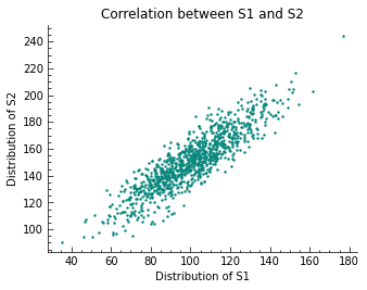
As designed, the two samples S1 and S2 are positively correlated with one another, as visualized in the scatter plot. It must be said that all the methods mentioned in this article only explain the linear part of the statistical relationship between random variables.
Covariance
To quantify the relationship between to variables that have a linear relationship, the empirical covariance is often used. It is calculated as the average of the product between the values from each sample, where the values have been centered (had their means subtracted). The calculation of the sample covariance is done using the following formula:
\[cov_{XY} := \frac{1}{n} \sum_{i=1}^{n} (\,x_{i} - \bar{x})\, (\,y_{i} - \bar{y})\, \iff\,\, \overline{xy} - \bar{x} \bar{y}\]$n$ is the number of values. Given the scatter plot of all $\left(x_{i},y_{i}\right)$ tuples with $x_{i}\in\mathrm{S1}$ and $y_{i}\in\mathrm{S2}$, a positive value for $cov(\,x,y)\,$ is expected. The relationship between the two distributions is of linear nature and so the covariance should be a good measure for how they are correlated.
cv = cov(S1, S2)
cv
array([[383.54554143, 375.65364293],
       [375.65364293, 467.25326789]])
The covariance matrix values of ~375.65 show that there is a strong positive correlation between S1 and S2. A strong sign for Multicollinearity between the two distributions. This would have to be addressed before training a linear regression model, among others for example. Given the design, there was no problem with satisfying the prerequisites that need to be met, in order for the covariance to be a good measurement for the relationship between two or more distributions found in a dataset (on a per-pair testing basis). Generally, explanatory variables are tested in this regard.
Pearson Correlation Coefficient
Another frequently used measure to determine whether 2 random variables are correlated or not and if, how strongly, is the empirical correlation coefficient, also known as the Pearson correlation coefficient. It utilizes the covariance value and divides it by the product of the standard deviations of the random variables. It is given by:
\[r_{XY} := \frac{cov_{XY}}{s_{X}s_{Y}}\]The domain of $r$ is $[-1,1]$, with:
| value $r$ | counterpart | bivariate relationship |
|---|---|---|
| 0 | - | none |
| 0.1 | -0.1 | weak |
| 0.3 | -0.3 | moderate |
| 0.5 | -0.5 | strong |
| 1 | -1 | perfect |
The plot of the values of two random variables ranges from close to a line with a negative slope, to close to a line with a positive slope. Values of $r\le-0.5$ and $r\ge0.5$ tend to signal a strong correlation in the respective direction. One of the good characteristics that $r$ has, is that its value does not change, if the random variables are subjected to a linear transformation. That means that the scale of the random variables or the difference in scale do not affect its value. The sign of $r$ is the same as for $cov$, a difference is that it is normed to the domain of $[-1,1]$
Unlike the $cov$ which returned a value of ~375.65 for our example.
Hypothesis Testing
In the next section, the pearsonr function from scipy is used to compute $r$
for the example. We conclude with a hypothesis test, asking whether random
variables S1 and S2 are positively correlated.
from numpy.random import seed
from scipy.stats import pearsonr

seed(42)
# calculate values
corr, p = pearsonr(S1, S2)
print(f'The Pearson correlation coefficient for S1 and S2 is {corr}\n')
# significance given p value and 0.05 threshold α
alpha = 0.05
if p > 0.05:
	print(f'p-value of {p} is greater alpha={alpha}, H0 is kept.')
else:
	print(f'p-value of {p} is smaller alpha={alpha} and H0 is rejected.\nThere is correlation between the two, given threshold alpha={alpha} on a one-tailed test.')
The Pearson correlation coefficient for S1 and S2 is 0.8873663623612615

p-value of 0.0 is smaller alpha=0.05 and H0 is rejected.
There is correlation between the two, given threshold alpha=0.05 on a one-tailed test.
The results show that the positive linear relationship between the random variables S1 and S2 was confirmed by $r$. The two metrics $r$ and $cov$ gave correct predictions in regard to the correlation.
This marks the end of this educational article. Thank you very much for reading it. Please feel free to link to this article or write a comment in the comments section below.
© Tobias Klein 2023 · All rights reserved
LinkedIn: https://www.linkedin.com/in/deep-learning-mastery/