Fundamental Concepts of Stochastic Gradient Descent Explained

A comprehensive exploration of the mathematical foundations of Stochastic Gradient Descent, crucial for understanding its application in optimization algorithms in deep learning.

Tags: optimization-algorithms mathematical-fundamentals gradient-descent algorithmic-understanding deep-learning-basics

Category: Deep Learning

Fundamental Concepts of Stochastic Gradient Descent Explained

Delving into Stochastic Gradient Descent.

This article delves into the fundamental concept of Stochastic Gradient Descent, elucidating the basic principles from which this optimization algorithm is derived. Among the topics covered in this article are:

Elements of a univariate linear function.
Understanding weights in this framework.
An introduction to Linear Regression.
The concept of empirical loss and the use of \(\mathit{L}_2\) loss.
An overview of Gradient Descent.

kletob · Article Summary: The math behind stepping the weights

Unraveling Univariate Linear Regression

At its core, a basic linear regression function is employed in various machine learning and statistical modeling applications. Conceptually, it represents a single straight line, defined mathematically by two real-valued parameters: \(w_{0},\,w_{1}\). Here, \(w_{0}\) is the intercept of the function, while \(w_{1}\) represents the slope of the regression line, collectively referred to as weights. The independent variable is usually denoted as \(x\), or \(x_{i}\,i\, \in \mathit{I}\) when referencing individual elements. The dependent variable is symbolized by \(y\), and the linear regression itself is expressed as \(h_{w}(\,x)\,\). The function is represented as:

\[h_{w}(\,x)\, =\, w_{1}x\,+\,w_{0}\]

Linear regression optimizes this function, particularly when dealing with \(n\) training points in the x,y plane. The algorithm aims to find the best fit for \(h_{w}\) based on these data points, adjusting \(w_{0}\) and \(w_{1}\) to minimize empirical loss.

Optimizing the \(L_{2}\) Loss

In scenarios where the noise in the dependent variable \(y_{j}\) follows a normal distribution, a squared-error loss function is typically the most effective for identifying optimal values for \(w_{0}\) and \(w_{1}\) within the constraints of linear regression. Assuming normally distributed noise for the dependent variable, the \(L_{2}\) loss function is employed. The loss is calculated by summing over all training data points:

\[\begin{aligned} \mathit{Loss}(\,h_{w})\,=\,&\sum_{j=1}^{N}\,\mathit{L}_{2}(\,y_{j},\,h_{w}(\,x_{j})\,) \\ \iff\, &\sum_{j=1}^{N}\,(\,y_{j}\, -\, h_{w}(\,x_{j})\,)^2 \\ \iff\, &\sum_{j=1}^{N}\,(\,y_{j}\, -\,(\,w_{1}x{j}\, +\, w_{0})\,)^2\, \end{aligned}\]

From Loss Function To Optimization

from sklearn.linear_model import LinearRegression
import numpy as np
import pandas as pd
import matplotlib.pyplot as plt
from torch import tensor

%matplotlib inline

Univariate Linear Regression

df = pd.read_csv("houses.csv").drop(columns="Unnamed: 0")
df.sample(n=10)

	Price	Size	Lot
9	123500	1161	9626
4	160000	2536	9234
7	145000	1572	12588
5	85000	2368	13329
12	156000	2240	21780
6	85000	1264	8407
16	182000	1320	15768
13	146500	1269	11250
0	212000	4148	25264
18	125000	1274	13634

Given price, size of the house and lot, we eliminate lot, so that there is only one independent variable (size).

df_indep = df["Size"].to_numpy()
df_dep = df["Price"].to_numpy()

We create a linear regression model that uses ordinary least squares for optimization by minimizing \(\mathit{L}_{2}\), using the implementation in the sklearn machine learning library. reg.score gives the global minimum for the \(\mathit{L}_{2}\) loss that one achieves using the optimal values for reg.coef_ and reg.intercept_. \(\mathit{L}_{2}\) is defined for a single training example, using pred for the model’s prediction and dep for the value of the dependent variable that the model tries to predict using the independent variable and the parameters:

\[\mathit{L}_{2}(\,\mathit{pred},\mathit{dep})\, =\, (\,\mathit{pred}\, -\, \mathit{dep})^2\]

After the model is fitted, the .score attribute gives the minimum value of the loss function using the \(\mathit{L}_2\) loss.

reg = LinearRegression(fit_intercept=True, n_jobs=-1).fit(
    df_indep.reshape(-1, 1), df_dep
)
reg.score(df_indep.reshape(-1, 1), df_dep)

0.4689809992584135

reg.coef_ gives the optimal value for the slope parameter, while reg.intercept_ gives the optimal value for the intercept parameter.

w1 = reg.coef_
w0 = reg.intercept_

print(
    f"The optimal value for the slope parameter is: {w1},\nwhile {w0} is the optimal value for the intercept."
)

The optimal value for the slope parameter is: [48.19930529],
while 64553.68328966276 is the optimal value for the intercept.

The function hw is a generic univariate linear regression function that makes the code more reproducible.

def hw(x, w1, w0):
    return w1 * x + w0

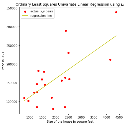
Plot Of A Univariate Regression Model

The plot below, shows training examples for independent and dependent variable and the linear regression line, using the optimal parameters.

fig, ax = plt.subplots(1, 1, figsize=(6, 6), tight_layout=True)
x_vals = np.linspace(min(df_indep) + 10, max(df_indep) + 5, 1000)
ax.scatter(df_indep, df_dep, c="r", label="actual x,y pairs")
ax.plot(x_vals, hw(x_vals, w1, w0), c="y", label="regression line")
ax.set_xlabel("Size of the house in square feet")
ax.set_ylabel("Price in USD")
plt.title("Ordinary Least Squares Univariate Linear Regression using $$L_{2}$$")
plt.legend(loc="best")
plt.show()

Plot Of The Loss Surface

Next, we plot the loss surface for \(\mathit{L}_{2}\). The convex shape of it is very important, as will be discussed.

def plotls(x, w1, w0):
    slope = np.linspace(w1 - 0.5 * w1, w1 + 0.5 * w1, 20)
    bias = np.linspace(w0 - 0.5 * w0, w0 + 0.5 * w0, 20)
    w1, w0 = np.meshgrid(slope, bias)
    loss = np.power((hw(df_indep, w1, w0) - df_dep), 2)
    fig = plt.figure(figsize=(10, 10))
    ax = fig.gca(projection="3d")
    surface = ax.plot_surface(
        w0,
        w1,
        loss,
        label="$$\mathit{L}_{2}$$ loss surface",
        cmap="viridis",
        edgecolor="none",
    )
    surface._facecolors2d = surface._facecolor3d
    surface._edgecolors2d = surface._edgecolor3d
    ax.set_xlabel("w1 - slope")
    ax.set_ylabel("w0 - bias")
    plt.legend(loc="best")

The loss function is convex and thus, always has a global minimum.

plotls(df_indep, w1, w0)

Solving By Hand

The loss function has a gradient of 0, where the minimum is found. The equation, that has to be solved, fulfills \(w_{opt}\, =\, \mathrm{Min}\,\mathit{Loss}_{w}( \,h_{w})\,\). The sum \(\sum_{j=1}^{N}\,(\,y_{j}\, - (\,w_{1}x_{j}\, + w_{0})\,) ^2\) is minimized, when its partial derivatives with respect to \(w_{0}\) and \(w_ {1}\) are zero. \(\begin{aligned}&\frac{\partial{h_{w}}}{\partial{w_{0}}}\, \sum_{j=1}^{N}\, (\,y_{j} - (\, w_ {1}x_{j}\, + w_{0})\,)^2 \,= 0 \\ \mathrm{and}\,\, &\frac{\partial{h_ {w}}}{\partial{w_{1}}}\, \sum_{j=1}^{N}\, (\,y_{j} - (\, w_{1}x_{j}\, + w_{0}) \,)^2\, = 0 \end{aligned}\)

Solving for \(w_{1}\) and \(w_{0}\) respectively, gives:

\[\begin{aligned}&w_{1}\, =\, \frac{\mathit{N}\,(\,\sum_{j=1}^{N}\, x_{j}y_{j})\, - (\,\sum_ {j=1}^{N}\,x_{j})\,(\,\sum_{j=1}^{N}\, y_{j})\,}{\mathit{N}(\,\sum_{j=1}^{N}\,x_ {j}^2)\, - (\,\sum_{j=1}^{N}\, x_{j})^2} \\ &w_{0}\, =\, \frac{(\,\sum_{j=1}^N y_{i} - w_{1}\,(\,\sum_{j=1}^{N}x_{j})\,)\,}{\mathit{N}} \end{aligned}\]

We plug in the values for the independent and dependent variables and solve for \(w_{1}\) and \(w_{0}\) respectively. Two functions are defined, one for each parameter.

def w1_solve(indep, dep):
    N = len(indep)
    nom = N * np.array(df_indep * df_dep).sum() - (
        np.array(indep).sum() * np.array(dep).sum()
    )
    denom = N * np.array(np.power(indep, 2).sum()) - np.array(
        np.power(np.array(indep).sum(), 2)
    )
    opt = nom / denom
    return opt


def w0_solve(indep, dep):
    N = len(indep)
    nom = dep.sum() - (w1_solve(indep, dep) * (np.array(indep).sum()))
    denom = N
    opt = nom / denom
    return opt

Solving for the slope parameter using w1_solve.

w1_solve(df_indep, df_dep)

48.19930529470915

In the same way, we use w0_solve to solve for \(w_{0}\).

w0_solve(df_indep, df_dep)

64553.683289662775

The optimal values for \(w_{0}\) and \(w_{1}\) that we gained from solving manually are the same as the ones that LinearRegression calculated for the two parameters. This is confirmed using np.allclose.

rig = [w0, w0_solve(df_indep, df_dep), w1, w1_solve(df_indep, df_dep)]

def allclose(rig):
    print(np.allclose(rig[0], rig[1]))
    print(np.allclose(rig[2], rig[3]))

allclose(rig)

True
True

Summary: Univariate Linear Model

The univariate linear model always has an optimal solution, where the partial derivatives are zero. However, this is not always the case, and the following algorithm for minimizing loss that does not depend on solving for zero values of the derivatives. It can be applied to any loss function. The Gradient Descent optimization algorithm is that optimizer. Its variation, the Stochastic Gradient Descent is widely used in deep learning to drive the training process.

Gradient Descent

The starting point for the Gradient Descent is any point in the weight space. Here that is a point in the \((\,w_{0},w_{1})\,\) plane. One then computes an estimate of the gradient and moves along the steepest gradient, during each step. This is repeated, until convergence is reached, which is not guaranteed in general. The point, on which convergence is reached can be a local minimum loss or a global one. In detail, while not converged, the Gradient Descent does the following:

Gradient Descent: Step

For each weight \(w_{i}\) in the set of all weights \(\mathbb{w}\), do for each step:

\[w_{i} = w_{i}\, - \alpha \frac{\partial}{\partial w_{i}}\, \mathit{Loss}( \,\mathbb{w})\,\]

Learning Rate

Parameter \(\alpha\) determines, how large each step size is. It is usually called Learning Rate. It is either a constant or decays over time or changes by layer.

Single Training Example

We calculate the partial derivatives, using the chain rule, and a single pair of independent and dependent variable \((x,y)\).

\[\frac{\partial}{\partial w_{i}}\mathit{Loss}(\,\mathbb{w})\, = \, \frac{\partial}{\partial w_{i}}(\,y\,-h_{w}(\,x)\,)^2 \, =\, 2(\,y\, - h_{w}( \,x)\,)\, \frac{\partial}{\partial w_{i}} (\,y - (\,w_{1}x + w_{0})\,)\,\]

The partial derivative was not specified for the ‘inner function’, since it depends on which of the two \(w\) parameters is parsimoniously derived.

The partial derivatives to \(w_{0}\), \(w_{1}\) are the following:

\[\frac{\partial}{\partial w_{0}}(\,y - (\,w_{1}x + w_{0})\,)\, = \frac{\partial}{\partial w_{0}} (\,y - w_{1}x - w_{0})\, =\, -1\] \[\frac{\partial}{\partial w_{1}}(\,y - (\,w_{1}x + w_{0})\,)\, = \frac{\partial}{\partial w_{1}} (\,y - w_{1}x - w_{0})\, =\, -x\]

Thus, the partial derivative of the loss function for \(w_{0}\) and \(w_{1}\) is:

\[\begin{aligned}&\frac{\partial}{\partial w_{0}}\mathit{Loss}(\,\mathbb{w})\, = -2\,(\,y\, - h_ {w}(\,x)\,) \\ \mathrm{and}\,\, &\frac{\partial}{\partial w_{1}}\mathit{Loss}( \,\mathbb{w})\, = -2x\,(\,y\, - h_{w}(\,x)\,)\, \end{aligned}\]

With these equations calculated, it is possible to plug in the values in the pseudocode under ‘Gradient Descent: Steps’. The -2 is added to the learning rate.

\[w_{0}\,\leftarrow\,w_{0}\,+\,\alpha\,(\,y\, - h_{w}(\,x)\,) \,\,\mathrm{and}\,\, w_{1}\,\,\leftarrow\, w_{1}\,+ \alpha\,x\,(\,y\, - h_{w}( \,x)\,)\,\]

N Training Examples

In the case of \(N\) independent and dependent variable pairs, the equations for updating the weights, are:

\[w_{0}\,\leftarrow\,w_{0}\,+\,\alpha\,\sum_{j=1}^{N}(\,y_{j}\, - h_{w}(\,x_{j}) \,)\,\,\mathrm{and}\,\, w_{1}\,\leftarrow\, w_{1}\,+ \alpha\,\sum_{j=1}^{N}x_ {j}\,(\,y_{j}\, - h_{w}(\,x_{j})\,)\,\]

The aim is to minimize the sum of the individual losses.

Batch Gradient Descent

The equations for updating the weights are applied after each batch. A batch consists of a specified number of training examples that are loaded into memory at once. The batch gradient descent for univariate linear regression updates the weights after each batch. It is computationally expensive, since it sums over all \(N\) training examples for every step and there may be many steps, until the global minimum is reached. If \(N\) is equal to the number of total elements in the training set, then the step is called an epoch.

Stochastic Gradient Descent

The stochastic gradient descent or SGD is a faster variant. It randomly picks a small subset of training examples at each step, and updates the weights using the equation under heading ‘Single Training Example’. It is common that the SGD selects a minibatch of \(m\) out of the \(N\) examples. E.g., Given \(N=1\mathit{e}4\) and the minibatch size of \(m=1\mathit{e}2\), the difference in order of magnitude between \(N\) and \(m\) is 2, which equals a factor of 100 times less computationally expensive compared to the entire batch for each step.

Standard Error

The standard error of the mean (\(\:\:{\sigma}_{\tilde{X}}\:\:\)) is the standard deviation of the sample means from the population mean \(\mu\). As sample size increases, the distribution of sample means tends to converge closer together to cluster around the true population mean \(\mu\).

The standard error can be calculated with the following formula:

\[{\sigma}_{\tilde{X}}\, = \frac{\sigma}{\sqrt{N}}\]

Where \({\sigma}_{\tilde{X}}\) is the standard deviation of the sample mean (standard error), \({\sigma}\) the standard deviation of the population and \({\sqrt{N}}\) the square root of the sample size.

Therefore, the standard error grows by the root of the sample size. That means, that given a minibatch of \(m=100\) training examples and a batch size of \(N=10000\), the denominator, using \(N\) examples for each step is \(\sqrt{10000}\,=\,100\), while for the minibatch it is \(\sqrt{100}\,=\,10\).

That means that the SGD trades being 100 times less computationally expensive with a 10 times larger standard error for this example.

Summary

In this article, we started by introducing the function of a univariate linear regression model and explored its \(L_{2}\) loss function. We learned that it is always convex in the case of \(L_{2}\) being the loss function by plotting the loss surface. We went on to optimize it, using the ordinary least squares algorithm, and by hand as well. We did this by forming the partial derivatives for both parameters and solving for zero for each one. The values obtained for the parameters were their optima. This was confirmed when we compared the self-calculated optima with those of the ordinary least squares method.

The batch gradient descent algorithm was explained and in particular how it updates the weights during each step. We calculated the partial derivatives for the parameters and used them to show how the weights are updated during each step. The stochastic gradient descent was introduced and compared to the batch gradient descent.